3.3 Partial Derivatives as Slices

A surface has no single slope: stand on a hillside and the steepness depends on which way you face. Calculus handles this the way it handles everything — by reducing to a problem already solved. Freeze one variable and the surface collapses to a curve, and curves we know how to differentiate. Fix $y = b$ and the slice $z = f(x, b)$ is an ordinary one-variable graph; its derivative at $x = a$ is the partial derivative

$f_x(a, b) = \lim_{h \to 0} \frac{f(a+h,\, b) - f(a, b)}{h},$

the slope of the surface at $(a, b)$ in the $x$ -direction. Freezing $x = a$ instead gives $f_y(a, b)$ , the slope in the $y$ -direction. The figure makes both slices into objects you can drive.

A translucent dome-shaped surface, the elliptic paraboloid z = 4 - x squared over 2 - y squared over 3, with two thick curves lying on its skin: a red parabola running in the x-direction at the fixed depth y = b, and a green parabola running in the y-direction at the fixed position x = a. Slider b slides the red curve forward and back across the dome and slider a slides the green curve left and right; the two curves always cross at the single point (a, b) on the surface, and the slope of each curve at that crossing is the corresponding partial derivative. 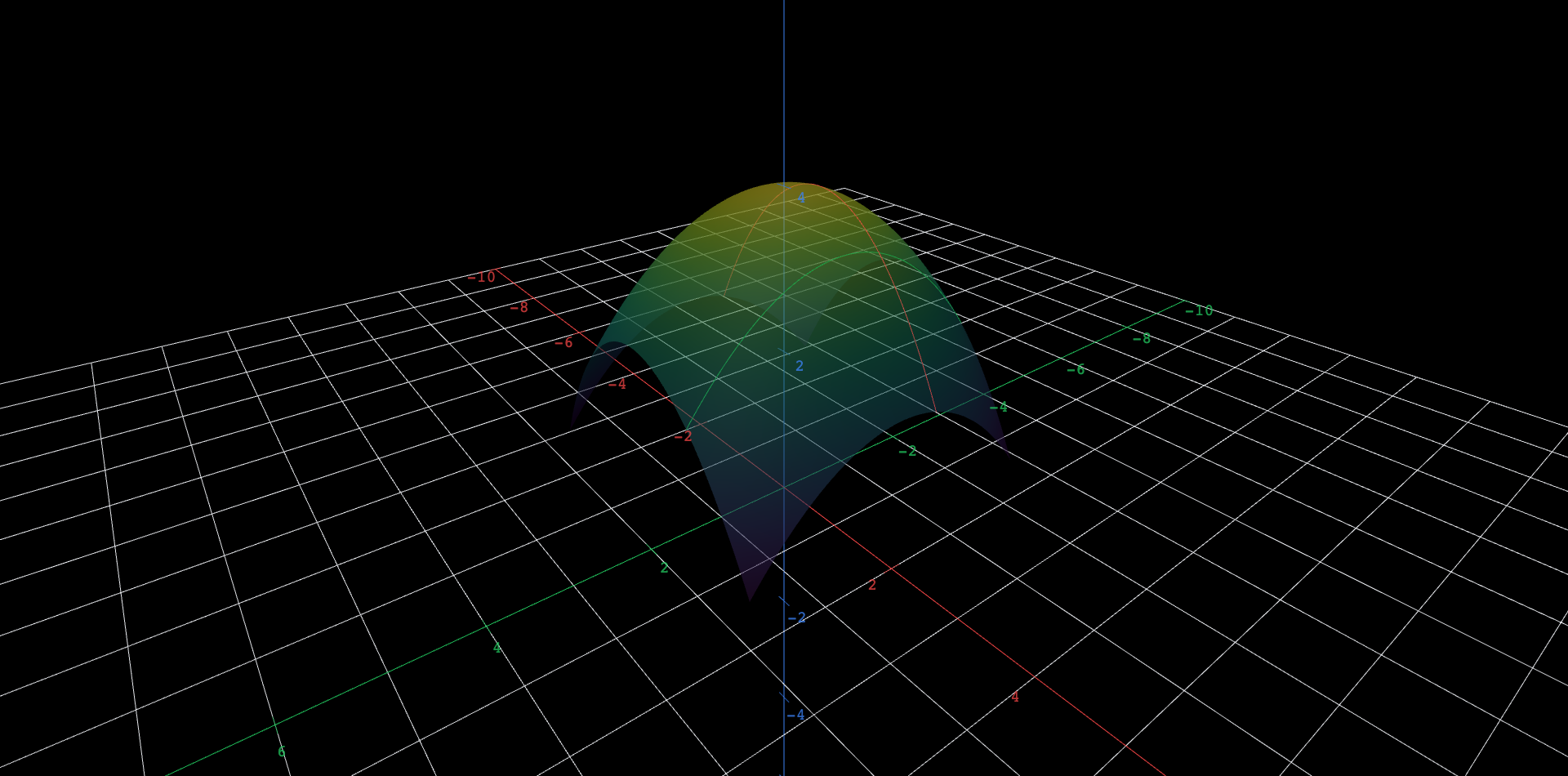— The translucent dome $z = 4 - x^2/2 - y^2/3$ with two thick curves lying on its skin: a red $x$ -direction slice at the fixed depth $y = b$ and a green $y$ -direction slice at the fixed position $x = a$ . Sliders $a$ and $b$ (each running $-2$ to $2$ , starting at $a = 1$ , $b = -0.5$ ) drag the two curves across the dome; they always cross at the single surface point $(a, b, f(a,b))$ , where the red curve's slope is $f_x$ and the green curve's slope is $f_y$ .

Explore

Orbit until you sight straight down the $y$ -axis, so the red slice flattens into a one-variable graph. What familiar curve is it? Now sight down the $x$ -axis and read the green slice the same way.
Drag the $b$ slider slowly from $-2$ to $2$ . The red curve sweeps across the dome — but watch its shape. Why does the parabola stay congruent to itself, only shifting in height? (Look at how $b$ enters $z = 4 - t^2/2 - b^2/3$ .)
One of the two slices is noticeably flatter than the other. Predict which from the expression — is it the $x^2/2$ or the $y^2/3$ term that makes a shallower parabola? — then orbit to check.
Set both sliders to $0$ . The two curves now crest together at the summit $(0, 0, 4)$ , and each has slope zero there. What does that pair of zero slopes say about the summit — and what will we call such points in the next chapter?
Return the sliders to $a = 1$ , $b = -0.5$ and zoom in on the crossing point. Decide the sign of each slope by eye: walking east (increasing $x$ ), does the red curve climb or fall? Walking north along the green curve? The example below puts numbers to both.

Differentiating with one eye closed

Computing a partial derivative needs no new rules: differentiate as in one-variable calculus, treating the frozen variable as a constant. The notation $\partial f/\partial x$ (or $f_x$ ) simply records which variable moved. Both partials together will feed everything that follows — tangent planes in the next section, the gradient in the next chapter — but each one, alone, is just the slope of a slice curve you could draw in Chapter 1 of any calculus book.

Example 1 Two slopes at one point of the dome

For $f(x, y) = 4 - x^2/2 - y^2/3$ , compute $f_x$ and $f_y$ , evaluate both at the scene's starting point $(a, b) = (1, -\tfrac{1}{2})$ , and check the signs against the figure.

Treat $y$ as a constant and differentiate in $x$ : the terms $4$ and $-y^2/3$ die, leaving $f_x = -x$ . Treat $x$ as a constant instead: $f_y = -\tfrac{2y}{3}$ . At $(1, -\tfrac{1}{2})$ :

$f_x(1, -\tfrac{1}{2}) = -1, \qquad f_y(1, -\tfrac{1}{2}) = -\tfrac{2}{3}\cdot\left(-\tfrac{1}{2}\right) = \tfrac{1}{3}.$

The crossing point sits at height $f(1, -\tfrac{1}{2}) = 4 - \tfrac{1}{2} - \tfrac{1}{12} = \tfrac{41}{12} \approx 3.42$ . So walking east from there, the red slice falls at one unit of height per unit of run ( $f_x = -1$ — the point is on the far side of the crest in $x$ ), while walking north the green slice climbs at a gentle $\tfrac{1}{3}$ ( $f_y > 0$ — the point sits south of the crest in $y$ , so north is uphill). Both signs match what the scene shows, and the size difference matches step 3: this dome is stiffer in $x$ than in $y$ .

-x

The red slice's slope: f_x of the dome ✓ Computed · mojocas 0.1.0 ✓ Agrees with the text

The example's first partial, computed: freeze $y$ and differentiate in $x$ , and the red slice's slope is $f_x = -x$ — at the scene's starting point $(1, -\tfrac{1}{2})$ that is $-1$ , the eastward fall.

-\frac{2}{3} \cdot y

The green slice's slope: f_y of the dome ✓ Computed · mojocas 0.1.0 ✓ Agrees with the text

The second partial, with $x$ frozen instead: $f_y = -2y/3$ , which at $(1, -\tfrac{1}{2})$ evaluates to $\tfrac{1}{3}$ — the gentle northward climb of the green slice.

An original work of XYZ Homework, built around interactive XYZ 3D figures. Aligned to OpenStax Calculus Volume 3 (Strang & Herman), © OpenStax (Rice University), licensed CC BY-NC-SA 4.0; no OpenStax content is reproduced, and this work is not affiliated with or endorsed by OpenStax or Rice University. License: CC-BY-NC-SA-4.0.