3.1 Contour Maps

A function of two variables assigns a height $z = f(x, y)$ to every point of the plane, and its graph is a landscape. Landscapes are hard to carry around, so hikers long ago invented something better: the map. A contour map of $f$ draws, on the flat plane, the level curves $f(x, y) = c$ for a list of equally spaced heights $c$ — each curve is the set of points where the landscape stands at exactly that height. The skill this section builds is fusion: seeing map and terrain as one object, so that a glance at crowded curves tells you "steep ground here" without any computation.

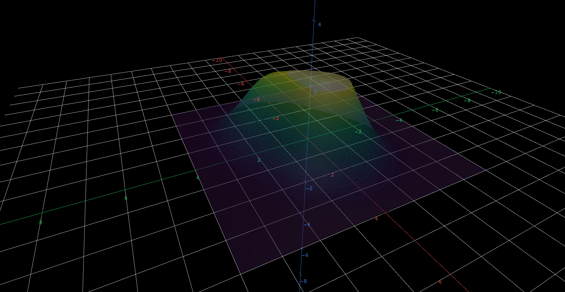
The figure stages the definition so you can run it in both directions. The landscape is a two-hill surface; the map is a separate object lying flat beneath it, and the map's altitude is under your control.

A half-transparent surface with two rounded hills of different heights — a taller one near (1, 0) and a shorter one near (-1, 1) — above a flat plane at z = 0 carrying twelve dark nested contour loops, two families of loops encircling the two hilltops. — The two-peak surface $z = 3e^{-((x-1)^2+y^2)/2} + 2e^{-((x+1)^2+(y-1)^2)/2}$ , half-transparent, above a flat sheet of twelve dark nested loops — a contour plot built from the same expression, resting at $z = 0$ but carrying a draggable z-offset, so the whole stack of level curves can ride up into the surface and seat itself, one loop at a time.

Explore

Orbit until you look straight down the $z$ -axis, so the contour plot reads as a flat map and the surface is only a colored blur behind it. From the map alone: how many peaks does this landscape have, and which one is taller? What about the map told you?
Still looking down, find where the loops crowd closest together and where they spread farthest apart. Then orbit to a side view and predict: walking through the crowded region, what would the ground feel like underfoot? Through the spread-out region?
Select the contour plot and drag its z-offset slowly upward from 0. Watch one outer loop until the rising sheet reaches the surface: the loop seats itself exactly where the plane cuts the landscape. Keep climbing. In what order do the loops land — and which peak runs out of loops to seat first?
Drag the z-offset back down until roughly half the loops are seated and half still float. Where seated loops stack tightly against the surface's wall — is that the crowded region you flagged in step 2?
Set the plot's Levels control from 12 up to 20. The levels are equally spaced in height, so what does tighter spacing on the map now say, precisely, about the surface between two neighboring curves?
Sketch, on paper, the map you expect for $4 - x^2 - y^2$ — the example below does the algebra — then edit both objects' expressions to it and look straight down. Where were the rings more crowded than you drew?

The map is the surface, disassembled

A level curve is a slice: cut the surface with the horizontal plane $z = c$ , and the cut edge, dropped straight down to the page, is the curve $f(x, y) = c$ . Dragging the z-offset runs this definition in reverse — the plane climbs, and at each height it re-seats the curve where the slice happens. Because the $c$ -values are equally spaced, the horizontal gap between neighboring curves is inversely tied to how fast $f$ climbs there: crowded curves mean steep ground.

The two-hill specimen shows what else a map encodes. The taller summit, near $(1, 0)$ , tops out around $3.16$ ; the shorter one, near $(-1, 1)$ , at about $2.25$ . Levels above $2.25$ therefore cut only the taller hill — which is why more loops encircle it. Counting rings compares summits.

Example 1 The rings of a paraboloid, before you plot them

For $g(x, y) = 4 - x^2 - y^2$ , find the level curves at $c = 3, 2, 1, 0$ and decide whether the rings crowd together or spread apart as you move outward from the center.

Setting $g = c$ gives $x^2 + y^2 = 4 - c$ : a circle of radius $\sqrt{4 - c}$ , so the four levels are circles of radii

$\sqrt{1} = 1,\quad \sqrt{2} \approx 1.414,\quad \sqrt{3} \approx 1.732,\quad \sqrt{4} = 2.$

The gaps between successive rings, moving outward, are about $0.414$ , then $0.318$ , then $0.268$ — shrinking. The rings crowd as you move out, because the bowl steepens: along the ring of radius $r$ the height $4 - r^2$ falls at rate $2r$ , so the farther out you stand, the less horizontal run a one-unit drop requires. Most people sketch the rings evenly spaced; the map knows better, and now so do you.

An original work of XYZ Homework, built around interactive XYZ 3D figures. Aligned to OpenStax Calculus Volume 3 (Strang & Herman), © OpenStax (Rice University), licensed CC BY-NC-SA 4.0; no OpenStax content is reproduced, and this work is not affiliated with or endorsed by OpenStax or Rice University. License: CC-BY-NC-SA-4.0.