15.3 Fractal Dimension

In addition to visual self-similarity, fractals exhibit other interesting properties. For example, notice that each step of the Sierpinski gasket iteration removes one quarter of the remaining area. If this process is continued indefinitely, we would end up essentially removing all the area, meaning we started with a 2-dimensional area, and somehow end up with something less than that, but seemingly more than just a 1-dimensional line.

import numpy as np
import matplotlib.pyplot as plt

# Build a Sierpinski gasket as a cloud of points (the "chaos game"),
# then MEASURE its dimension by covering it with smaller and smaller boxes.
N_POINTS = 40000          # EDIT
SHAPE = "gasket"          # EDIT: "gasket", "square", or "segment"

rng = np.random.default_rng(7)
if SHAPE == "gasket":
    verts = np.array([[0.0, 0.0], [1.0, 0.0], [0.5, np.sqrt(3) / 2]])
    pts = np.zeros((N_POINTS, 2))
    cur = verts[0]
    for i, j in enumerate(rng.integers(0, 3, N_POINTS)):
        cur = (cur + verts[j]) / 2
        pts[i] = cur
elif SHAPE == "square":
    pts = rng.random((N_POINTS, 2))
else:
    pts = np.column_stack([rng.random(N_POINTS), np.full(N_POINTS, 0.5)])

sizes, counts = [], []
print(f"{'grid':>8}{'box size':>12}{'boxes hit N':>14}")
for k in range(2, 9):
    m = 2 ** k
    cells = {(int(x * m), int(y * m)) for x, y in pts}
    sizes.append(1 / m)
    counts.append(len(cells))
    print(f"{m:>6}^2{1 / m:>12.5f}{len(cells):>14,}")

logs, logn = np.log(1 / np.array(sizes)), np.log(counts)
slope, intercept = np.polyfit(logs, logn, 1)
exact = np.log(3) / np.log(2)
print(f"\nN grows like (1/size)^D, so D is the slope of log N against log(1/size)")
print(f"   measured D = {slope:.4f}")
if SHAPE == "gasket":
    print(f"   exact  D = log(3)/log(2) = {exact:.4f}   (a 2-D shape would give 2.0000)")

fig, (ax1, ax2) = plt.subplots(1, 2, figsize=(10, 4.2))
ax1.plot(pts[::10, 0], pts[::10, 1], ",", color="#1f4e79")
ax1.set_aspect("equal"); ax1.axis("off"); ax1.set_title(f"{SHAPE}: {N_POINTS:,} points")
ax2.plot(logs, logn, "o-", color="#b03a2e")
ax2.plot(logs, slope * logs + intercept, "--", color="gray")
ax2.set_xlabel("log(1 / box size)"); ax2.set_ylabel("log(boxes hit)")
ax2.set_title(f"slope = measured dimension = {slope:.3f}")
plt.tight_layout(); plt.show()
# Try it: set SHAPE = "square" (slope near 2) or "segment" (slope near 1).

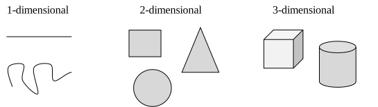
To explore this idea, we need to discuss dimension. Something like a line is 1-dimensional; it only has length. Any curve is 1-dimensional. Things like boxes and circles are 2-dimensional, since they have length and width, describing an area. Objects like boxes and cylinders have length, width, and height, describing a volume, and are 3-dimensional.

Three labelled groups of shapes illustrating dimension. Under 1-dimensional, a straight line segment and a wiggly curve. Under 2-dimensional, a shaded rectangle, a shaded circle and a shaded triangle. Under 3-dimensional, a shaded cube and a shaded cylinder.

Certain rules apply for scaling objects, related to their dimension.

If I had a line with length 1, and wanted scale its length by 2, I would need two copies of the original line. If I had a line of length 1, and wanted to scale its length by 3, I would need three copies of the original.

Three line segments illustrating how a 1-dimensional object scales, labelled 1, 2 and 3. The first is one unit long and undivided. The second is twice as long with one tick mark, showing it is made of 2 copies of the first. The third is three times as long with two tick marks, showing 3 copies.

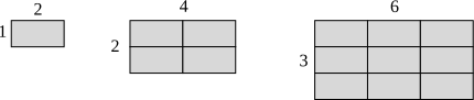
If I had a rectangle with length 2 and height 1, and wanted to scale its length and width by 2, I would need four copies of the original rectangle. If I wanted to scale the length and width by 3, I would need nine copies of the original rectangle.

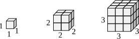
Three shaded rectangles illustrating how a 2-dimensional object scales. The first is labelled 1 tall by 2 wide. The second, scaled by 2, is labelled 2 by 4 and is gridded into 4 copies of the first. The third, scaled by 3, is labelled 3 by 6 and is gridded into 9 copies.

If I had a cubical box with sides of length 1, and wanted to scale its length, its width, and its height by 2, I would need eight copies of the original cube. If I wanted to scale the length, width, and height by 3, I would need 27 copies of the original cube.

Three cubes illustrating how a 3-dimensional object scales. The first has all three edges labelled 1. The second has edges labelled 2 and is divided into 8 copies of the first. The third has edges labelled 3 and is divided into 27 copies.

Notice that in the 1-dimensional case, copies needed = scale.

In the 2-dimensional case, copies needed $=$ scale $^{2}$ .
In the 3-dimensional case, copies needed $=$ scale $^{3}$ .

From these examples, we might infer a pattern.

Example 1

Use the scaling-dimension relation to determine the dimension of the Sierpinski gasket.

Show solution

Suppose we define the original gasket to have side length 1. The larger gasket shown is twice as wide and twice as tall, so has been scaled by a factor of 2.

Notice that to construct the larger gasket, 3 copies of the original gasket are needed.

Using the scaling-dimension relation $C = S^{D},$ we obtain the equation $3 = 2^{D}$

since $2^{1} = 2$ and $2 squared equals 4,$ we can immediately see that $D$ is somewhere between 1 and $2;$ the gasket is more than a 1 -dimensional shape, but we've taken away so much area its now less than 2-dimensional.

Solving the equation $3 = 2^{D}$ requires logarithms. If you studied logarithms earlier, you may recall how to solve this equation (if not, just skip to the box below and use that formula):

$\begin{matrix} 3 = 2^{D} & Take the logarithm of both sides \\ \log (3) = \log (2^{D}) & Use the exponent property of logs \\ \log (3) = D \log (2) & Divide by log(2) \\ D = \frac{\log (3)}{\log (2)} \approx 1.585 & The dimension of the gasket is about 1.585 \end{matrix}$

Note

Scaling-Dimension Relation, to find Dimension

To find the dimension $D$ of a fractal, determine the scaling factor $S$ and the number of copies $C$ of the original shape needed, then use the formula

import math

# (name, copies C needed, scaling factor S).  EDIT this table and re-run.
SHAPES = [("line segment", 2, 2),
          ("filled square", 4, 2),
          ("solid cube", 8, 2),
          ("Sierpinski gasket", 3, 2),
          ("Koch curve", 4, 3),
          ("Sierpinski carpet", 8, 3),
          ("Cantor set", 2, 3),
          ("Menger sponge", 20, 3)]

print(f"{'shape':<20}{'copies C':>10}{'scale S':>9}{'C = S^D':>22}{'D':>9}")
for name, C, S in SHAPES:
    D = math.log(C) / math.log(S)
    print(f"{name:<20}{C:>10}{S:>9}{f'{C} = {S}^D':>22}{D:>9.4f}")

print("\nwhy the gasket's dimension cannot be a whole number")
C, S = 3, 2
print(f"   we need {C} = {S}^D")
lo, hi = math.floor(math.log(C, S)), math.ceil(math.log(C, S))
print(f"   {S}^{lo} = {S ** lo} is too small, {S}^{hi} = {S ** hi} is too big")
print(f"   so D sits strictly between {lo} and {hi}: D = log({C})/log({S}) = "
      f"{math.log(C) / math.log(S):.4f}")
print(f"   check: {S}^{math.log(C) / math.log(S):.4f} = {S ** (math.log(C) / math.log(S)):.4f}")
print("   more than a line (it has infinite detail), less than an area (all area was removed)")

print("\nDIY: how many copies would you need to scale each shape by 4?")
for name, C, S in SHAPES:
    D = math.log(C) / math.log(S)
    print(f"   {name:<20} 4^{D:.4f} = {4 ** D:>10.2f} copies")
# Try it: add ("your fractal", C, S) using the copies and scale you counted by hand.

$D = \frac{\log (C)}{\log (S)}$

We will now turn our attention to another type of fractal, defined by a different type of recursion. To understand this type, we are first going to need to discuss complex numbers.

Adapted from Math in Society by David Lippman, hosted on LibreTexts (math.libretexts.org) and licensed under CC BY-SA 3.0. Changes were made. License: CC-BY-SA-3.0.