6.3 Least Squares: Beat the Normal Equations

Seven measurements: $(-2, -2, -2.4)$ , $(-2, 1, 0.5)$ , $(-1, -1, -0.9)$ , $(0, 0, 0.6)$ , $(1, -1, -0.3)$ , $(1, 2, 2.7)$ , $(2, 1, 2.2)$ . One model: a plane $z = ax + by + c$ . Each data point would like the coefficients to satisfy $a x_i + b y_i + c = z_i$ — and read that way, each measurement is a linear equation in the unknowns $(a, b, c)$ : seven planes in coefficient space. Chapter 1 says three independent planes already pin down a point, so seven generically share nothing. The system is overdetermined and inconsistent; no plane passes through all seven points, and the interesting question is which plane misses them least.

"Least" needs a score. The residual of point $i$ is the vertical gap $r_i = z_i - (a x_i + b y_i + c)$ , and the score is the sum of squared residuals over all seven points — squared so that misses above and below both count against you, and big misses count hardest. Your job in the first figure: tune $a$ , $b$ , $c$ by hand and drive the score as low as you can. Then find out whether you beat the machine. (You will not. The point is understanding why.)

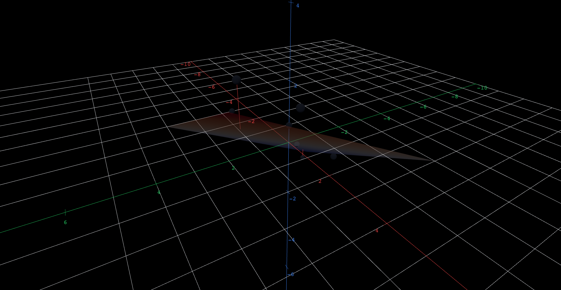
Seven small dark spheres scattered in 3D space around a tilted, semi-transparent plane through the origin. Two vertical dashed red segments connect two of the spheres to the plane, showing how far the plane misses them vertically. A second, better-fitting plane is included but hidden until the student reveals it. — Seven data points and the deliberately imperfect starting plane $z = 0.5x + 0.5y$ . The dashed red segments at $(1, 2)$ and $(-2, -2)$ are residuals — vertical gaps between point and plane. A least-squares plane is hidden in the scene; leave it hidden until you have a fit you are proud of.

Explore the figure

Orbit the data and read the two drawn residuals. Above $(1, 2)$ the plane sits at $z = 1.5$ while the point is at $2.7$ — a gap of $1.2$ above. At $(-2, -2)$ the plane is at $-2$ and the point at $-2.4$ — a gap of $0.4$ below.
Judge all seven points: five sit above the starting plane, only two below. A plane that splits its misses is doing better than one that is systematically low — this one is too low, and too flat in the $y$ direction. Its score is $3.55$ .
Hide the two objects labeled residual at $(1, 2)$ and residual at $(-2, -2)$ — they are drawn for the starting plane only and will not follow your edits. Then edit the plane's expression: try $0.5x + 0.9y + 0.3$ first, and watch the plane move as you retype. Better or worse? How can you tell from the picture alone?
Keep tuning — treat the three coefficients like three sliders and iterate until you cannot visibly improve. Hand fits usually land near $a \approx 0.4$ – $0.5$ , $b \approx 0.9$ – $1.0$ , $c \approx 0.3$ – $0.5$ , scoring somewhere between $0.1$ and $0.3$ . Write your three numbers down.
Now reveal the hidden object labeled least-squares plane and orbit. How close did you come — and can you find any single coefficient change that would visibly improve on it?

The normal equations

Your tuning loop was a search of a subspace. Collect the seven heights a candidate plane produces into a vector in $\mathbb{R}^7$ : it equals $a$ times the column of $x_i$ 's, plus $b$ times the column of $y_i$ 's, plus $c$ times a column of ones. As $(a, b, c)$ range over all values, these vectors sweep out the span of three columns — a three-dimensional subspace of $\mathbb{R}^7$ — and you were hunting the point of it closest to the data vector $\mathbf{z} = (z_1, \dots, z_7)$ . Section 6.1 answered that hunt in general: closest means the residual vector $(r_1, \dots, r_7)$ is perpendicular to the subspace, i.e. to each of the three spanning columns. Writing out those three dot products — $\sum x_i r_i = 0$ , $\sum y_i r_i = 0$ , $\sum r_i = 0$ — and substituting the definition of $r_i$ gives the normal equations:

$15a + 6b - c = 11.5, \qquad 6a + 12b = 14.1, \qquad -a + 7c = 2.4$

\begin{bmatrix}15 & 6 & -1 \\ 6 & 12 & 0 \\ -1 & 0 & 7\end{bmatrix}

The normal equations' left side, from the data ✓ Computed · mojocas 0.1.0 ✓ Agrees with the text

Where those nine coefficients come from. Stack the seven measurements into a $7 \times 3$ matrix $A$ — a column of $x_i$ , a column of $y_i$ , a column of ones — and the three dot-product conditions are exactly $A^{\mathsf{T}}A$ , computed here from the measurements themselves rather than summed by hand.

\begin{bmatrix}\frac{23}{2} \\ \frac{141}{10} \\ \frac{12}{5}\end{bmatrix}

The normal equations' right side, from the data ✓ Computed · mojocas 0.1.0 ✓ Agrees with the text

And the three numbers on the right: $A^{\mathsf{T}}\mathbf{z}$ , the same seven measurements dotted against the same three columns. Between this and the matrix above, every number in the system is now derived from the data — so a slip in one of the twelve dot-product sums would stop the build rather than quietly solve the wrong system correctly.

Three equations, three unknowns, one solution — the whole search compressed onto an index card.

Example 1 Solve the normal equations

Solve the system above and compute the winning coefficients to four decimal places.

The second equation gives $b = (14.1 - 6a)/12$ and the third gives $c = (2.4 + a)/7$ . Substituting both into the first: $15a + (14.1 - 6a)/2 - (2.4 + a)/7 = 11.5$ . Multiplying through by $14$ : $210a + 7(14.1 - 6a) - 2(2.4 + a) = 161$ , so $210a + 98.7 - 42a - 4.8 - 2a = 161$ , giving $166a = 67.1$ and $a = 0.4042$ . Back-substituting, $b = 1.175 - 0.5(0.4042) = 0.9729$ and $c = (2.4 + 0.4042)/7 = 0.4006$ . The machine's plane is $z = 0.4042x + 0.9729y + 0.4006$ — compare it with the hidden plane you revealed, and with your own hand fit. (In exact arithmetic $a = 671/1660$ , $b = 323/332$ , $c = 133/332$ ; the four-place decimals are these fractions rounded.)

\begin{bmatrix}1 & 0 & 0 & \frac{671}{1660} \\ 0 & 1 & 0 & \frac{323}{332} \\ 0 & 0 & 1 & \frac{133}{332}\end{bmatrix}

The normal equations, reduced ✓ Computed · mojocas 0.1.0 ✓ Agrees with the text

The three normal equations as an augmented matrix, reduced to solved form by a computer algebra system. The final column is the winning plane in exact arithmetic: $a = \tfrac{671}{1660}$ , $b = \tfrac{323}{332}$ , $c = \tfrac{133}{332}$ — the fractions that round to the $0.4042$ , $0.9729$ , $0.4006$ worked out above.

The winner scores $0.0723$ — nearly fifty times better than the starting plane's $3.55$ , and better than any hand fit. Its seven residuals are $-0.046$ , $-0.065$ , $+0.077$ , $+0.199$ , $-0.132$ , $-0.051$ , $+0.018$ : small everywhere, mixed in sign, and summing to zero — the visible face of the perpendicularity conditions, since $\sum r_i = 0$ is literally one of them.

Feel the trade-off

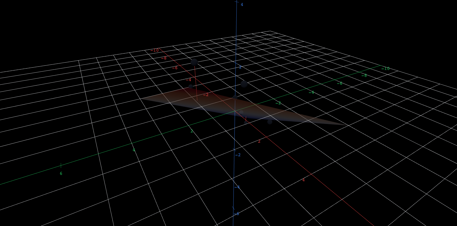
The second figure replays the contest with the coefficients on actual sliders and the two residual segments now live — they stretch and shrink as you drag.

Seven small dark spheres scattered in 3D space around a tilted, semi-transparent plane. Three sliders named a, b, and c control the plane z = ax + by + c. Two vertical dashed red segments connect two of the spheres to the plane and stretch or shrink live as the sliders move. A second, better-fitting plane is included but hidden. — The same seven data points, with the plane $z = ax + by + c$ driven by sliders $a$ , $b$ , $c$ and the dashed residual segments at $(1, 2)$ and $(-2, -2)$ updating live as you drag. The least-squares plane is hidden in this scene too.

From the starting setting $(0.5, 0.5, 0)$ , drag $b$ upward and watch the residual at $(1, 2)$ shrink — then watch what your improvement costs at $(-2, -2)$ . Every coefficient helps some points at other points' expense; that tension is what the score arbitrates.
Try to make both drawn residuals small at once, then check the rest of the data by orbiting. The best reachable setting on these sliders is about $(0.40, 0.95, 0.40)$ , scoring $0.0800$ — the true optimum lies between slider clicks, and no setting the sliders can reach attains $0.0723$ .
Reveal the hidden least-squares plane and set the sliders to hug it as closely as you can. At the optimum, no single-slider move improves the score: each slider direction has been made exactly perpendicular to the remaining error. That is the normal equations, felt by hand.

An original work of XYZ Homework, built around interactive XYZ 3D figures. Its chapter sequence is aligned to Interactive Linear Algebra (Margalit & Rabinoff, Georgia Tech, GNU FDL); this work is original, copies nothing from it, and is not affiliated with or endorsed by its authors. License: CC-BY-NC-SA-4.0.