5.5 Stochastic Matrices and the Steady State

The last section ended on a rule: the largest eigenvalue decides the long run. Almost always that means growth without bound or decay to nothing. The interesting case is the one where the largest eigenvalue is exactly $1$ — the long run then goes somewhere and stays.

Model a system that is always in one of three states, and let the numbers $M_{i j}$ be the probability of moving to state $i$ given that you are currently in state $j$ . Take

$M equals open parenthesis 0.6, 0.3, 0.2; 0.4, 0.5, 0.2; 0, 0.2, 0.6 close parenthesis$

Read the columns: from state 1, the chances of going to states 1, 2, 3 are $0.6$ , $0.4$ , $0$ — you never jump from state 1 to state 3 in a single step. Each column sums to $1$ , because from wherever you are you must end up somewhere. A matrix with non-negative entries whose columns each sum to $1$ is called stochastic.

A distribution $𝐱 equals open parenthesis x sub 1, x sub 2, x sub 3 close parenthesis$ records the probability of being in each state; its entries are non-negative and sum to $1$ , so distributions form a triangle inside the plane $x + y + z = 1$ . Applying $M$ advances the system one step, and the column condition is exactly what guarantees the result is another distribution — the entries of $M 𝐱$ sum to $1$ whenever $𝐱$ 's do.

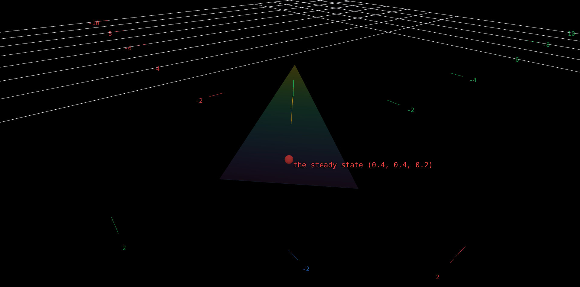
A small semi-transparent sloping triangle, the set of all probability distributions over three states, with a dashed dark line marking one edge of the triangle where the third probability is zero. A short thick green marker shows the chosen starting distribution, set by two independent sliders - it is a genuine distribution, and sits on the triangle, only while the two slider values sum to at most one; past that the third probability goes negative and the marker leaves the triangle, and an amber arrow runs from it to where one step of the chain sends it. A red dot marks the steady state at (0.4, 0.4, 0.2). Wherever the start is placed, the amber arrow points toward the red dot, and when the start is dialed onto the red dot the arrow shrinks to nothing. — The plane of distributions, with the dashed dark line marking one edge of the triangle where genuine distributions live. The green marker is the starting distribution $(s, a, 1 - s - a)$ set by the two sliders, the amber arrow runs from it to where one step of the chain sends it, and the red dot is the steady state $open parenthesis 0.4, 0.4, 0.2 close parenthesis$ .

Explore the figure

At the defaults $s equals 0.1$ , $a equals 0.1$ — a system almost certainly in state 3 — the amber arrow is long. One step takes this start to $open parenthesis 0.25, 0.25, 0.5 close parenthesis$ , a displacement of $(+ 0.15, + 0.15, - 0.30)$ : probability is draining out of state 3 and splitting evenly between states 1 and 2.
Drag the sliders to $s equals 0.4$ , $a equals 0.4$ . The arrow shrinks to nothing. That is the steady state: one step changes it not at all, which is what "steady" means.
Move a little away from those values in any direction. The arrow reappears, and it points back toward the red dot. Every start is pulled the same way.
Try a corner, $s equals 1$ , $a equals 0$ — the system definitely in state 1. One step gives $open parenthesis 0.6, 0.4, 0 close parenthesis$ , which is still on the edge where state 3 has probability zero: the arrow runs along that edge rather than into the interior, because $M$ has a $0$ in the row-3, column-1 position and you cannot reach state 3 from state 1 in a single step. Take a second step and the interior opens up; the destination is unchanged either way.

The steady state is an eigenvector

A distribution that a step leaves alone satisfies $M π = π$ — which is the eigenvector equation for eigenvalue $1$ . Finding it means solving $(M - I) π = 0$ , so the steady state is simply the null space of $M - I$ , with one extra condition to pin down the scale: its entries must sum to $1$ .

Why should $λ equals 1$ be available at all? Because the columns of $M$ each sum to $1$ , the columns of $M - I$ each sum to $0$ . That is a dependency among the rows: adding all three rows of $M - I$ gives the zero row. Dependent rows means a determinant of zero, which means $M - I$ is not invertible, which means its null space contains something other than $0$ . Every stochastic matrix has $1$ as an eigenvalue, and the argument used nothing about the particular numbers.

Be careful about what that buys. It produces a nonzero vector fixed by $M$ , and no more. Nothing in the determinant forces that vector's entries to be non-negative, or even to sum to something other than zero so that it could be rescaled to sum to $1$ — and a fixed vector failing either test is not a distribution. That every stochastic matrix does in fact fix a genuine distribution is a separate and harder theorem (Perron–Frobenius), which this book takes on trust. What the argument above settles is the easy half: that there is something to look for.

0

M - I is singular, as it must be ✓ Computed · mojocas 0.1.0 ✓ Agrees with the text

The determinant of $M - I$ is exactly zero. This is not a numerical coincidence of the chosen entries: the columns of $M$ sum to $1$ , so the columns of $M - I$ sum to $0$ , and a matrix whose columns sum to zero has dependent rows. So $λ equals 1$ is guaranteed before any of it is computed — though, as the text notes, turning the fixed vector that guarantees into an honest distribution takes a theorem this determinant does not supply.

[\begin{matrix} 1 & 0 & - 2 \\ 0 & 1 & - 2 \\ 0 & 0 & 0 \end{matrix}]

Reducing to find it ✓ Computed · mojocas 0.1.0 ✓ Agrees with the text

The reduced form of $M - I$ : two pivots and one free variable, so the null space is a line. Reading it off, $x sub 1 equals 2 x sub 3$ and $x sub 2 equals 2 x sub 3$ , so every solution is a multiple of $open parenthesis 2, 2, 1 close parenthesis$ . Those three numbers sum to $5$ , so dividing by $5$ gives the one solution that is a distribution.

That division is the last step: $π = \frac{1}{5} (2, 2, 1) = (0.4, 0.4, 0.2)$ , the red dot. Confirm it directly, since the check is short. The first coordinate of $M π$ is $0.6 (0.4) + 0.3 (0.4) + 0.2 (0.2) = 0.24 + 0.12 + 0.04 = 0.4$ , and the other two work out the same way.

Why everything drifts there

Existence is not convergence. What makes step 3 of the exploration true — that every start is pulled in — is the rest of the spectrum. The eigenvalues of $M$ are $1$ , $\frac{1}{2}$ and $\frac{1}{5}$ . They are distinct, and eigenvectors belonging to distinct eigenvalues are always independent, so these three form a basis — which is exactly the situation the last section needed in order to write $A = P D P^{- 1}$ .

Write any starting distribution in that basis. Its $λ equals 1$ component is some multiple of $π$ , and the other two components lie along the remaining eigenvectors. Applying $M$ a total of $k$ times multiplies those pieces by $1 to the power k$ , $(\frac{1}{2})^{k}$ and $(\frac{1}{5})^{k}$ . The first piece never moves; the other two shrink by a factor of one half and one fifth at every step, vanishing as $k$ grows. Since the sums stay equal to $1$ throughout, the surviving piece must be $π$ itself. So

$M^{k} 𝐱 ⟶ π for every starting distribution 𝐱$

and the rate is governed by the second-largest eigenvalue, $\frac{1}{2}$ : the distance to the steady state roughly halves each step. That is why the amber arrow is long far from the red dot and short near it.

Example 1 Two steps, and how much is left

Starting from complete certainty about state 1 — the distribution $open parenthesis 1, 0, 0 close parenthesis$ — compute the distribution after one step and after two, and compare each with the steady state.

One step reads the first column of $M$ directly, since $M open parenthesis 1, 0, 0 close parenthesis$ selects it: the result is $open parenthesis 0.6, 0.4, 0 close parenthesis$ .

Two steps means applying $M$ to that. First coordinate: $0.6 (0.6) + 0.3 (0.4) + 0.2 (0) = 0.36 + 0.12 = 0.48$ . Second: $0.4 (0.6) + 0.5 (0.4) + 0.2 (0) = 0.24 + 0.20 = 0.44$ . Third: $0 (0.6) + 0.2 (0.4) + 0.6 (0) = 0.08$ . So after two steps the distribution is $open parenthesis 0.48, 0.44, 0.08 close parenthesis$ , and it does still sum to $1$ .

Now compare with $π equals open parenthesis 0.4, 0.4, 0.2 close parenthesis$ . The start was off by $(0.6, - 0.4, - 0.2)$ ; after one step, off by $open parenthesis 0.2, 0, minus 0.2 close parenthesis$ ; after two steps, off by $open parenthesis 0.08, 0.04, minus 0.12 close parenthesis$ . The error is shrinking by roughly a half each time, matching the second eigenvalue $\frac{1}{2}$ — and it is shrinking regardless of the fact that the start was as far from the steady state as a distribution can get.

An original work of XYZ Homework, built around interactive XYZ 3D figures. Its chapter sequence is aligned to Interactive Linear Algebra (Margalit & Rabinoff, Georgia Tech, GNU FDL); this work is original, copies nothing from it, and is not affiliated with or endorsed by its authors. License: CC-BY-NC-SA-4.0.