5.3 Complex Eigenvalues and the Spiral

Some matrices turn every direction. The cleanest examples are the rotation–scaling matrices: rotate the plane by an angle $b$, then scale it by a factor $a > 0$. Written out, this map sends $(x, y)$ to $$(a\cos b \; x - a\sin b \; y, \;\; a\sin b \; x + a\cos b \; y)$$. If $\sin b \ne 0$, every nonzero vector is rotated by the full angle $b$ — no line is invariant, no real eigenvector exists, and the hunts of the last two sections come home empty. The misalignment function never touches zero.

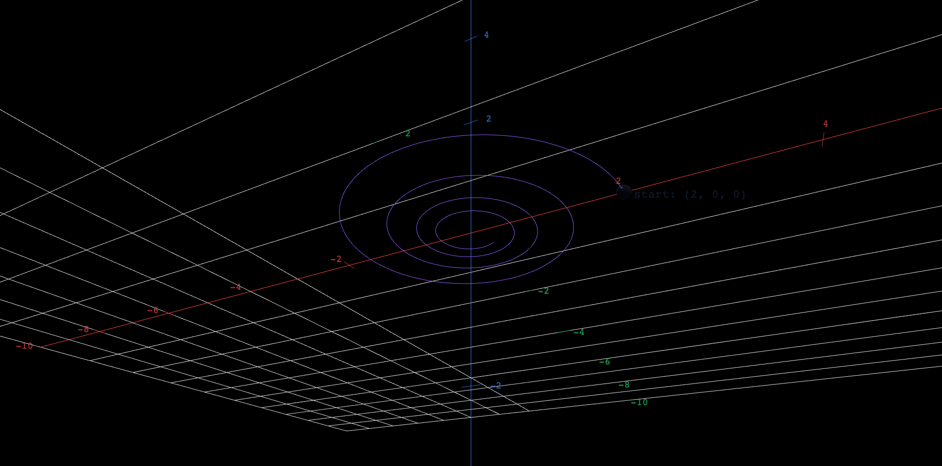
Yet the matrix still has structure, and the way to see it is to iterate. Start at the point $(2, 0)$ and apply the matrix over and over. Each application multiplies the distance from the origin by $a$ and advances the angle by $b$, so after $k$ steps the point sits at $2a^k(\cos kb, \; \sin kb)$. Letting the step count run continuously traces the curve $2a^t(\cos bt, \; \sin bt)$ — the violet spiral in the figure, with the iteration's start marked at $(2, 0, 0)$.

Explore in 3D (opens in a new tab)

Explore the figure

1. At the defaults, follow the curve from the marked start point. With $b = 0.6$ it wraps around the origin about $3.8$ times over the run, and with $a = 0.96$ each unit of time shaves four percent off the radius, ending near radius $0.4$. Rotation and decay, superimposed.
2. Set $a = 1$. The spiral closes into a perfect circle of radius $2$: pure rotation, nothing gained or lost. This is the knife-edge between decay and growth.
3. Push $a$ to $1.04$. The same curve now unwinds outward, finishing near radius $9.6$. A four-percent difference per step, compounded forty times, is the whole difference between collapse and explosion.
4. Return $a$ to $0.96$ and sweep $b$ across its range. At $b = 0.2$ the path barely completes one lap; at $b = 1.2$ it wraps nearly eight times. Notice what $b$ never changes: the radius at each time depends on $a$ alone.

Every direction, tested at once

The spiral follows one starting point. To see that no direction survives, test them all together: hand the whole unit circle to the matrix and watch where it goes.

Interactive figureA rotation-scaling turns every directionDrag the growth factor a and rotation angle b sliders.

▶ Explore interactively

XYZ Graph · viewer build 5edf91b

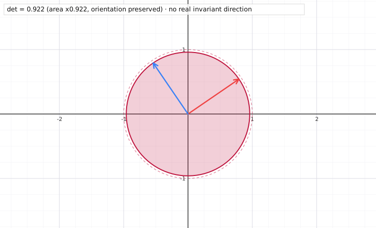
1. At the defaults the image circle is barely smaller than the dashed one: $a = 0.96$ takes four percent off every radius, in every direction equally. Compare with the spiral, which spends forty steps making that same four percent visible.
2. Watch the two colored arrows. They are the images of $(1, 0)$ and $(0, 1)$, and both have swung off their axes by the same angle $b$. A rotation-scaling plays no favorites among directions.
3. Notice what is missing. In the previous section's figure two dashed lines marked the directions the matrix could not turn. Here there are none — not hidden, not faint: absent, because with $\sin b \ne 0$ no real direction is left invariant.
4. Now drag $b$ to $0$. The rotation stops and the arrows snap back onto the axes: $A$ is $a$ times the identity, so every direction is invariant. Nothing new is drawn — and that is worth pausing on, because the figure looks the same as it did a moment ago while meaning the opposite. Two dashed lines are absent at $b = 0.6$ because no direction survives, and absent at $b = 0$ because every direction does; a picture cannot draw infinitely many lines any more than it can draw none meaningfully. The readout is what separates them, and it changes as you cross $b = 0$.

Eigenvalues without eigenvectors

The eigenvalue machinery does not break here — it reports complex numbers. The characteristic polynomial of the rotation–scaling matrix is

$$\lambda^2 - 2a\cos b \,\lambda + a^2 = 0$$

and its discriminant is $4a^2\cos^2 b - 4a^2 = -4a^2\sin^2 b$, which is negative whenever $\sin b \ne 0$: no real roots, confirming what the pictures showed. The roots are the complex pair $\lambda = a\cos b \pm i\,a\sin b$, better read in polar form as $\lambda = a e^{\pm i b}$. The two sliders of the figure are literally the two coordinates of the eigenvalue: $a$ is its modulus and $b$ is its argument. A complex eigenvalue does not mark an invariant line; it prescribes a motion — turn by the argument, scale by the modulus, once per application — and the spiral is that prescription traced out in time. The trichotomy you explored is the modulus test: $|\lambda| < 1$ spirals in, $|\lambda| = 1$ circles, $|\lambda| > 1$ spirals out.

An original work of XYZ Homework, built around interactive XYZ 3D figures. Its chapter sequence is aligned to Interactive Linear Algebra (Margalit & Rabinoff, Georgia Tech, GNU FDL); this work is original, copies nothing from it, and is not affiliated with or endorsed by its authors. License: CC-BY-NC-SA-4.0.