1.4 Free Variables and Parametric Form

The previous section made elimination safe: every row operation trades one plane for another plane through the same intersection, so reducing a system never disturbs its solutions. Safety is only half the job. Once a system is fully reduced you still have to read the answer off it, and when the answer is larger than a single point, reading it off requires a form we have not yet written down.

Start with a system so small that it is already reduced — a single equation in three unknowns:

$x - y + 2 z = 2$

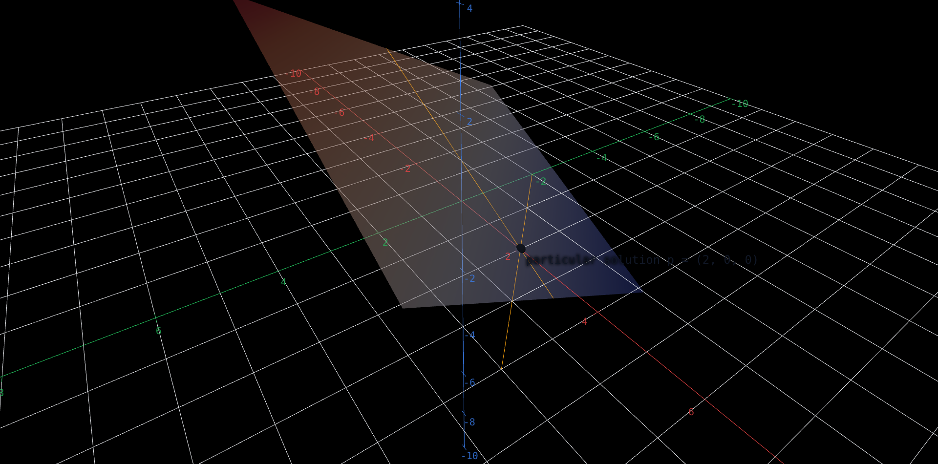
Its augmented matrix is the one row $open parenthesis 1, minus 1, 2 ∣ 2 close parenthesis$ , and there is nothing to eliminate: no second row exists to clear anything against. The leading $1$ sits in the $x$ column, which makes $x$ a pivot variable. No leading entry appears in the $y$ column or the $z$ column, so $y$ and $z$ are free variables — free in the strict sense that you may assign them any values you like, whereupon the equation dictates what $x$ must be. Three unknowns against one real constraint should leave two degrees of freedom, and it does: the solution set is a plane. The figure draws that plane along with a machine for naming its points.

Explore the figure

Start at $s equals 0$ , $a equals 0$ . The two amber lines cross exactly on the black dot at $open parenthesis 2, 0, 0 close parenthesis$ ; check it in the equation: $2 - 0 + 2 (0) = 2$ . That is the solution you get by setting both free variables to zero.
Drag $s$ to $1$ . The crossing slides to $open parenthesis 3, 1, 0 close parenthesis$ , travelling along the red line — the direction the solution moves when only $y$ is changed. Confirm: $3 - 1 + 0 = 2$ .
Now drag $a$ to $1$ as well. The crossing lands on $open parenthesis 1, 1, 1 close parenthesis$ : raising $z$ by one has forced $x$ down by two, which is exactly what the blue direction $open parenthesis minus 2, 0, 1 close parenthesis$ records. Confirm: $1 - 1 + 2 = 2$ .
Set $a equals 1$ and sweep $s$ across its whole range. The crossing runs from $(- 2, - 2, 1)$ to $open parenthesis 2, 2, 1 close parenthesis$ , staying on the drawn sheet the whole way — an entire line of solutions at one fixed height. Two sliders, two independent directions of travel: the solution set is a plane, not a line.

Reading the answer off the pivot

A reduced row asks you to do exactly one thing: solve it for its pivot variable. Here that gives

$x = 2 + y - 2 z$

Now hand the free variables names of their own. Write $y = s$ and $z = a$ — the two sliders — and every solution of the equation is

$(x, y, z) = (2 + s - 2 a, s, a)$

Splitting that into the part carrying no parameter and the parts carrying $s$ and $a$ turns it into the parametric form:

$(x, y, z) = (2, 0, 0) + s (1, 1, 0) + a (- 2, 0, 1)$

Every piece of this has a job. The vector $open parenthesis 2, 0, 0 close parenthesis$ is a particular solution: one point that works, obtained by switching both free variables off. The other two are directions, and what qualifies them is that each solves the homogeneous version of the equation, $x - y + 2 z = 0$ . For $open parenthesis 1, 1, 0 close parenthesis$ : $1 - 1 + 0 = 0$ . For $open parenthesis minus 2, 0, 1 close parenthesis$ : $- 2 - 0 + 2 = 0$ . A vector that changes the left-hand side by zero can be added to any solution without breaking it, which is why sliding $s$ or $a$ never lifts the crossing point off the sheet.

Notice also that the naming is exact rather than merely generous. The second and third coordinates of the parametric form are the parameters, so distinct pairs $(s, a)$ give distinct points and every point of the plane is produced once. The free variables have become coordinates on the solution set. Solving the same equation for $z$ instead would give $z = 1 - 0.5 x + 0.5 y$ , the graph form the figure renders as a surface; it describes the identical set, but only parametric form survives when there is no single variable you can conveniently isolate.

open bracket 1, minus 1, 2, 2 close bracket

Already as reduced as it gets ✓ Computed · mojocas 0.1.0 ✓ Agrees with the text

The augmented matrix of $x - y + 2 z = 2$ handed to a computer algebra system for reduction — and returned unchanged, because there is nothing left to do. One row, one pivot, and it sits in the $x$ column. Of the three variable columns, two carry no pivot, and those two are the free variables: $3$ unknowns minus $1$ pivot leaves the $2$ parameters the figure puts on sliders.

An equation that says nothing

Nothing in that argument depended on the system having only one equation, and it is worth seeing why. Add a second equation, $2 x - 2 y + 4 z = 4$ , and reduce the pair. Subtracting twice the first row from the second turns $open parenthesis 2, minus 2, 4 ∣ 4 close parenthesis$ into $open parenthesis 0, 0, 0 ∣ 0 close parenthesis$ . A row of zeros is the equation $0 equals 0$ : true, and true at every point of space, so it excludes nothing. The reduced system still has one pivot and two free variables, and its solution set is still the plane you have been sweeping. The second equation was a multiple of the first — geometrically, the same plane written twice.

open bracket 1, minus 1, 2, 2; 0, 0, 0, 0 close bracket

A redundant row reduces to zeros ✓ Computed · mojocas 0.1.0 ✓ Agrees with the text

Two equations in, one equation out. The reduced matrix's second row is entirely zero, so the second equation imposed no condition the first had not already imposed. The lesson is a counting one: the number of equations is not the number of constraints — the number of pivots is. Here that count is $1$ either way, and $3 - 1 = 2$ free variables survive.

Example 1 Name a point, and name it only once

The point $open parenthesis 1, 1, 1 close parenthesis$ satisfies $x - y + 2 z = 2$ . Find the values of $s$ and $a$ that produce it, and explain why no other pair could.

In the parametric form $(x, y, z) = (2 + s - 2 a, s, a)$ the last two coordinates are the parameters themselves: $y = s$ and $z = a$ . The point has $y equals 1$ and $z equals 1$ , so $s equals 1$ and $a equals 1$ , with no choice made anywhere. Checking the first coordinate confirms the fit: $2 + 1 - 2 (1) = 1$ , which is the $x$ we wanted. As a combination, $(2, 0, 0) + 1 (1, 1, 0) + 1 (- 2, 0, 1) = (1, 1, 1)$ . Uniqueness is not luck; it follows from the shape of the form. Because the parameters are read directly off two coordinates, different pairs $(s, a)$ can never collide, and since any point of the plane supplies its own $y$ and $z$ , every point is reached. The parameterization is therefore a genuine coordinate system on the solution set, not merely a device for manufacturing solutions — which is what lets you dial the sliders to $s equals 1$ , $a equals 1$ and land on this point exactly.

An original work of XYZ Homework, built around interactive XYZ 3D figures. Its chapter sequence is aligned to Interactive Linear Algebra (Margalit & Rabinoff, Georgia Tech, GNU FDL); this work is original, copies nothing from it, and is not affiliated with or endorsed by its authors. License: CC-BY-NC-SA-4.0.