While behavior of ODEs at singular points is more complicated, certain singular points are not especially difficult to solve. Let us look at some examples before giving a general method. We may be lucky and obtain a power series solution using the method of the previous section, but in general we may have to try other things.
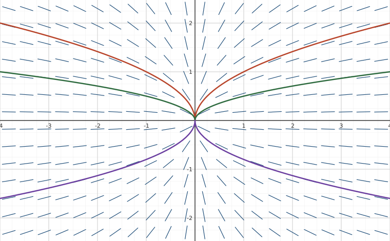
Interactive figureSlope field of x y' = r y at the singular point x = 0, with the exponent r on a sliderDrag the Frobenius exponent r slider from -2 to 2.
XYZ Graph · viewer build 5edf91b
The slope field of x y′ = r y with three of its solutions y = C|x|^r drawn through it. The equation worked just below, 2xy′ − y = 0, is the case r = 1/2 — where the figure opens — because substituting y = x^r turns the ODE into the indicial equation for r. Drag the slider to watch the singular point change character: for r < 0 the solutions themselves blow up at x = 0; at r = 0 they flatten into the horizontal lines y = C; for 0 < r < 1, the range containing Lebl's r = 1/2, they reach the origin with a vertical tangent, which is why the trivial y = 0 is the only solution differentiable there; at r = 1 the two branches meet in a corner; and only for r > 1 do they arrive with zero slope and the singular point stop hurting.
Not every problem with a singular point has a solution of the form , of course. But perhaps we can combine the methods. What we will do is to try a solution of the form
where is an analytic function.
Method of Frobenius
Before giving the general method, let us clarify when the method applies. Let
be an ODE. As before, if , then is a singular point. If, furthermore, the limits
both exist and are finite, then we say that is a regular singular point.
Let us now discuss the general Method of Frobenius1. Let us only consider the method at the point for simplicity. The main idea is the following theorem.
The method usually breaks down like this.
We seek a Frobenius-type solution of the form We plug this into equation (7.3.7). We collect terms and write everything as a single series.
The obtained series must be zero. Setting the first coefficient (usually the coefficient of ) in the series to zero we obtain the indicial equation, which is a quadratic polynomial in .
If the indicial equation has two real roots and such that is not an integer, then we have two linearly independent Frobenius-type solutions. Using the first root, we plug in and we solve for all to obtain the first solution. Then using the second root, we plug in and solve for all to obtain the second solution.
If the indicial equation has a doubled root , then there we find one solution and then we obtain a new solution by plugging into Equation (7.3.7) and solving for the constants .
If the indicial equation has two real roots such that is an integer, then one solution is and the second linearly independent solution is of the form where we plug into (7.3.7) and solve for the constants and .
Finally, if the indicial equation has complex roots, then solving for in the solution results in a complex-valued function---all the are complex numbers. We obtain our two linearly independent solutions2 by taking the real and imaginary parts of .
The main idea is to find at least one Frobenius-type solution. If we are lucky and find two, we are done. If we only get one, we either use the ideas above or even a different method such as reduction of order (Exercise 2.1.8) to obtain a second solution.
Bessel Functions
An important class of functions that arises commonly in physics are the Bessel functions3. For example, these functions appear when solving the wave equation in two and three dimensions. First we have Bessel's equation of order :
We allow to be any number, not just an integer, although integers and multiples of are most important in applications. When we plug
into Bessel's equation of order we obtain the indicial equation
Therefore we obtain two roots and . If is not an integer following the method of Frobenius and setting , we obtain linearly independent solutions of the form
Bessel functions will be convenient constant multiples of and . First we must define the gamma function
Notice that . The gamma function also has a wonderful property
From this property, one can show that when is an integer, so the gamma function is a continuous version of the factorial. We compute:
We define the Bessel functions of the first kind of order and as
As these are constant multiples of the solutions we found above, these are both solutions to Bessel's equation of order . The constants are picked for convenience.
When is not an integer, and are linearly independent. When is an integer we obtain
In this case it turns out that
and so we do not obtain a second linearly independent solution. The other solution is the so-called Bessel function of second kind. These make sense only for integer orders and are defined as limits of linear combinations of and as approaches in the following way:
As each linear combination of and is a solution to Bessel's equation of order , then as we take the limit as goes to , is a solution to Bessel's equation of order . It also turns out that and are linearly independent. Therefore when is an integer, we have the general solution to Bessel's equation of order
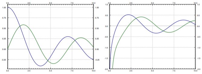
for arbitrary constants and . Note that goes to negative infinity at . Many mathematical software packages have these functions and defined, so they can be used just like say and . In fact, they have some similar properties. For example, is a derivative of , and in general the derivative of can be written as a linear combination of and . Furthermore, these functions oscillate, although they are not periodic. See Figure for graphs of Bessel functions.
Figure : Plot of the and in the first graph and and in the second graph.
Footnotes
[1] Named after the German mathematician Ferdinand Georg Frobenius (1849 – 1917).
[2] See Joseph L. Neuringera, The Frobenius method for complex roots of the indicial equation, International Journal of Mathematical Education in Science and Technology, Volume 9, Issue 1, 1978, 71–77.
[3] Named after the German astronomer and mathematician Friedrich Wilhelm Bessel (1784 – 1846).
These eBooks are a prerelease and are not yet certified conformant with WCAG 2.1 AA or ADA Title II. Every page is built against an automated accessibility gate, and the published editions will meet ADA Title II requirements when they release in late September 2026. If something is unusable, please tell us.