Many functions can be written in terms of a power series
If we assume that a solution of a differential equation is written as a power series, then perhaps we can use a method reminiscent of undetermined coefficients. That is, we will try to solve for the numbers . Before we can carry out this process, let us review some results and concepts about power series.
Definition
As we said, a power series is an expression such as
(7.1.1)
where and are constants. Let
denote the so-called partial sum. If for some , the limit
exists, then we say that the series (7.1.1) converges at . Note that for , the series always converges to . When (7.1.1) converges at any other point , we say that (7.1.1) is a convergent power series. In this case we write
If the series does not converge for any point , we say that the series is divergent.
Radius of Convergence
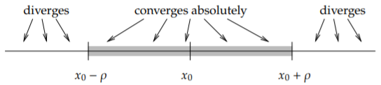
If a power series converges absolutely at some , then for all such that (that is, is closer than to ) we have for all . As the numbers sum to some finite limit, summing smaller positive numbers must also have a finite limit. Hence, the series must converge absolutely at .
Figure : Convergence of a power series.
See Figure . In Example the radius of convergence is as the series converges everywhere. In Example the radius of convergence is . We note that is another way of saying that the series is divergent. A useful test for convergence of a series is the ratio test. Suppose that
is a series such that the limit
exists. Then the series converges absolutely if and diverges if .
Let us apply this test to the series (7.1.1). That is we let in the test. Compute
Define by
Then if the series (7.1.1) converges absolutely. If , then the series always converges. If , then the series converges absolutely if , and diverges if . That is, the radius of convergence is .
A similar test is the root test. Suppose
exists. Then converges absolutely if and diverges if . We can use the same calculation as above to find . Let us summarize.
The root or the ratio test does not always apply. That is the limit of or might not exist. There exist more sophisticated ways of finding the radius of convergence, but those would be beyond the scope of this chapter. The two methods above cover many of the series that arise in practice. Often if the root test applies, so does the ratio test, and vice versa, though the limit might be easier to compute in one way than the other.
Analytic Functions
Functions represented by power series are called analytic functions. Not every function is analytic, although the majority of the functions you have seen in calculus are. An analytic function is equal to its Taylor series1 near a point . That is, for near we have
(7.1.2)
where denotes the derivative of at the point .
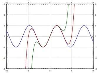
Figure : The sine function and its Taylor approximations around of and degree.
For example, sine is an analytic function and its Taylor series around is given by
In Figure we plot and the truncations of the series up to degree 5 and 9. You can see that the approximation is very good for near 0, but gets worse for further away from 0. This is what happens in general. To get a good approximation far away from you need to take more and more terms of the Taylor series.
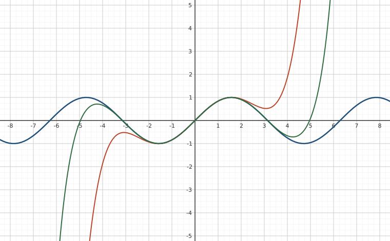
Interactive figureSine and its degree-5 and degree-9 Taylor polynomials about a movable pointDrag the Expansion point x0 slider from -6 to 6.
XYZ Graph · viewer build 5edf91b
The book's sine picture with the expansion point set free: sin x in blue, its degree-5 Taylor polynomial in red and its degree-9 in green, both taken about x₀ = a. It opens at a = 0, the book's own picture; drag a along the sine curve and watch the sharp accuracy window slide with it — degree 9 always reaching further than degree 5, both failing at a distance, and the failure region moving rigidly with the centre.
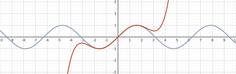
Interactive figureHow far out does degree n reach?Drag the degree n slider from 1 to 15.
XYZ Graph · viewer build 5edf91b · plotted curve with n = 9 checked against “Sine's Taylor polynomial through degree 9, computed” (mojocas 0.1.0): agrees
The figure above reproduces the book's Figure 2 — degrees 5 and 9, about a centre you can move. This one pins the centre at 0 and puts the DEGREE on the slider instead. Degree 1 is the line x, useful only at the origin. Each step adds one term and pushes the agreement outward: by degree 5 the rust curve holds the first hump, by degree 9 (the highest truncation drawn above) it tracks the wave to about x = 4, and at degree 15 it stays with it nearly to the frame's edge. What never changes is the shape of the failure — every truncation is a polynomial, so it must eventually run off to infinity. The degree only decides how far out it agrees first.Sine's Taylor polynomial through degree 9, computed ✓ Computed · mojocas 0.1.0✓ Agrees with the text Sine's Taylor polynomial through degree 9, computed, computed exactly by mojocas 0.1.0, and confirmed to agree with the result stated in the text.The section states sine's Taylor series about 0 in closed form; written out to degree 9 it is exactly this polynomial, and the computer algebra system derives it from sin(x) itself rather than from the formula. These are the same coefficients the figure above plots — and on every rebuild the plotted polynomial, with its degree slider fixed at 9, is checked against this computed series, which is in turn checked against the text's formula. So the curve you drag and the series the text asserts really are checked against one another.
Manipulating Power Series
One of the main properties of power series that we will use is that we can differentiate them term by term. That is, suppose that is a convergent power series. Then for in the radius of convergence we have
Notice that the term corresponding to disappeared as it was constant. The radius of convergence of the differentiated series is the same as that of the original.
Convergent power series can be added and multiplied together, and multiplied by constants using the following rules. First, we can add series by adding term by term,
We can multiply by constants,
We can also multiply series together,
where . The radius of convergence of the sum or the product is at least the minimum of the radii of convergence of the two series involved.
Power Series for Rational Functions
Polynomials are simply finite power series. That is, a polynomial is a power series where the are zero for all large enough. We can always expand a polynomial as a power series about any point by writing the polynomial as a polynomial in . For example, let us write as a power series around :
In other words , , , and all other . To do this, we know that for all as the polynomial is of degree 2.
We write , we expand, and we solve for , , and . We could have also differentiated at and used the Taylor series formula (7.1.2).
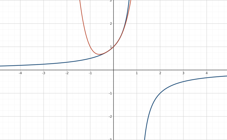
Let us look at rational functions, that is, ratios of polynomials. An important fact is that a series for a function only defines the function on an interval even if the function is defined elsewhere. For example, for we have
This series is called the geometric series. The ratio test tells us that the radius of convergence is . The series diverges for and , even though is defined for all .
Interactive figureGeometric series against 1/(1 - x), with the number of terms on a sliderDrag the Highest power kept slider from 0 to 24.
XYZ Graph · viewer build 5edf91b
1/(1 − x) in blue, the partial sum Sₙ = 1 + x + ⋯ + xⁿ in red. Drag n: the red curve locks onto the blue one across (−1, 1) and nowhere else — exactly the radius of convergence 1 this section derives. Past x = 1 the partial sum climbs off the top of the frame while 1/(1 − x) runs calmly along the lower right, still perfectly well defined. Left of x = −1 the partial sum flies apart, and watch its direction: it flips from up to down at every single step of n, because the terms alternate. At x = −1 itself it neither converges nor blows up — it just hops 1, 0, 1, 0, never settling on the value 1/2 the function has there.
We can use the geometric series together with rules for addition and multiplication of power series to expand rational functions around a point, as long as the denominator is not zero at . Note that as for polynomials, we could equivalently use the Taylor series expansion (7.1.2).
Footnotes
[1] Named after the English mathematician Sir Brook Taylor (1685–1731).
These eBooks are a prerelease and are not yet certified conformant with WCAG 2.1 AA or ADA Title II. Every page is built against an automated accessibility gate, and the published editions will meet ADA Title II requirements when they release in late September 2026. If something is unusable, please tell us.