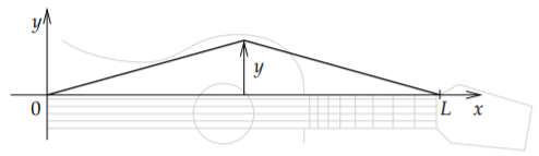
Consider a guitar string of length . We studied this setup in Section 4.7. Let be the position on the string, the time, and the displacement of the string. See Figure .
Figure : Vibrating string.
The problem is governed by the equations
(5.3.1)
We saw previously that the solution is of the form
where and were determined by the initial conditions. The natural frequencies of the system are the (circular) frequencies for integers .
But these are free vibrations. What if there is an external force acting on the string. Let us assume say air vibrations (noise), for example a second string. Or perhaps a jet engine. For simplicity, assume nice pure sound and assume the force is uniform at every position on the string. Let us say as force per unit mass. Then our wave equation becomes (remember force is mass times acceleration)
(5.3.2)
with the same boundary conditions of course.
We want to find the solution here that satisfies the above equation and
(5.3.3)
That is, the string is initially at rest. First we find a particular solution of (5.3.2) that satisfies . We define the functions and as
We then find solution of (5.3.1). If we add the two solutions, we find that solves (5.3.2) with the initial conditions.
So the big issue here is to find the particular solution . We look at the equation and we make an educated guess
We plug in to get
or after canceling the cosine. We know how to find a general solution to this equation (it is a nonhomogeneous constant coefficient equation). The general solution is
The endpoint conditions imply . So
or , and also
Assuming that is not zero we can solve for to get
(5.3.4)
Therefore,
The particular solution we are looking for is
Now we get to the point that we skipped. Suppose that . What this means is that is equal to one of the natural frequencies of the system, i.e. a multiple of . We notice that if is not equal to a multiple of the base frequency, but is very close, then the coefficient in (5.3.4) seems to become very large. But let us not jump to conclusions just yet. When for even, then and hence we really get that . So resonance occurs only when both and . That is when for odd .
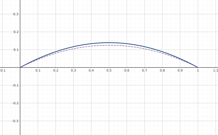
Interactive figureSteady periodic shape of the forced string as ω variesDrag the Forcing frequency ω slider from 0.2 to 13.
XYZ Graph · viewer build 5edf91b
The steady periodic shape X(x) of the forced string at t = 0, built from this section's worked example — F₀ = 1, L = 1, a = 1 — with its ω = 1 promoted to a slider. The dashed curve is the steady deflection x(1−x)/2 the string would hold under a constant load; drag ω down to 0.2 and X settles onto it. Drag upward instead and at ω = π the curve flies clean off the frame: resonance. Carry on to 2π, where sin(ωL/a) vanishes exactly as it did at π, and nothing happens — cos(ωL/a) = 1 there kills the numerator too, so the shape passes smoothly through as a shallow dip. 3π blows up again; 4π is quiet again. Resonance really does strike only at odd multiples of πa/L.
We could again solve for the resonance solution if we wanted to, but it is, in the right sense, the limit of the solutions as gets close to a resonance frequency. In real life, pure resonance never occurs anyway.
The above calculation explains why a string will begin to vibrate if the identical string is plucked close by. In the absence of friction this vibration would get louder and louder as time goes on. On the other hand, you are unlikely to get large vibration if the forcing frequency is not close to a resonance frequency even if you have a jet engine running close to the string. That is, the amplitude will not keep increasing unless you tune to just the right frequency.
Similar resonance phenomena occur when you break a wine glass using human voice (yes this is possible, but not easy1) if you happen to hit just the right frequency. Remember a glass has much purer sound, i.e. it is more like a vibraphone, so there are far fewer resonance frequencies to hit.
When the forcing function is more complicated, you decompose it in terms of the Fourier series and apply the above result. You may also need to solve the above problem if the forcing function is a sine rather than a cosine, but if you think about it, the solution is almost the same.
It is not hard to compute specific values for an odd extension of a function and hence (5.3.5) is a wonderful solution to the problem. For example it is very easy to have a computer do it, unlike a series solution. A plot is given in Figure .
Underground Temperature Oscillations
Let be the temperature at a certain location at depth underground at time . See Figure .
The temperature satisfies the heat equation , where is the diffusivity of the soil. We know the temperature at the surface from weather records. Let us assume for simplicity that
where is the yearly mean temperature, and is midsummer (you can put negative sign above to make it midwinter if you wish). gives the typical variation for the year. That is, the hottest temperature is and the coldest is . For simplicity, we will assume that . The frequency is picked depending on the units of , such that when , then . For example if is in years, then .
It seems reasonable that the temperature at depth will also oscillate with the same frequency. This, in fact, will be the steady periodic solution, independent of the initial conditions. So we are looking for a solution of the form
for the problem
(5.3.6)
We will employ the complex exponential here to make calculations simpler. Suppose we have a complex valued function
We will look for an such that . To find an , whose real part satisfies (5.3.6), we look for an such that
where . Note that so you could simplify to . Hence the general solution is
We assume that an that solves the problem must be bounded as since should be bounded (we are not worrying about the earth core!). If you use Euler’s formula to expand the complex exponentials, you will note that the second term will be unbounded (if ), while the first term is always bounded. Hence .
Furthermore, since . Thus . This means that
We will need to get the real part of , so we apply Euler’s formula to get
Then finally
Yay!
Notice the phase is different at different depths. At depth the phase is delayed by . For example in cgs units (centimeters-grams-seconds) we have (typical value for soil), . Then if we compute where the phase shift we find the depth in centimeters where the seasons are reversed. That is, we get the depth at which summer is the coldest and winter is the warmest. We get approximately centimeters, which is approximately feet below ground.
Be careful not to jump to conclusions. The temperature swings decay rapidly as you dig deeper. The amplitude of the temperature swings is . This function decays very quickly as (the depth) grows. Let us again take typical parameters as above. We will also assume that our surface temperature swing is Celsius, that is, . Then the maximum temperature variation at centimeters is only Celsius.
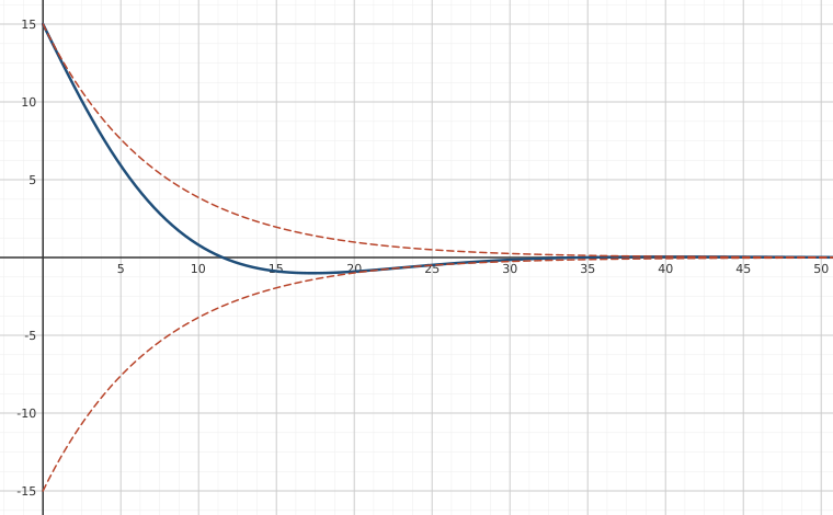
Interactive figureUnderground temperature versus depth through the yearDrag the Time of year (ωt) slider from 0 to 6.2832.
XYZ Graph · viewer build 5edf91b
The section's own solution — a surface swing of A₀ = 15 °C damped and phase-shifted by √(ω/2k) — plotted against depth in feet with the book's soil value k = 0.005, giving a decay constant of 0.136 per foot. Drag the time-of-year slider from midsummer (ωt = 0) to midwinter (ωt = π) and watch the warm band march downward: past about 12 ft the ground already sits on the opposite side of the axis from the surface, reaching full reversal near 23 ft — the flipped season the text describes. The dashed envelope is the amplitude: it has collapsed to the book's ±0.66 °C by 23 ft and is indistinguishable from zero by 50 ft, which is why a wine cellar works.
You need not dig very deep to get an effective “refrigerator,” with nearly constant temperature. That is why wines are kept in a cellar; you need consistent temperature. The temperature differential could also be used for energy. A home could be heated or cooled by taking advantage of the above fact. Even without the earth core you could heat a home in the winter and cool it in the summer. The earth core makes the temperature higher the deeper you dig, although you need to dig somewhat deep to feel a difference. We did not take that into account above.
Footnotes
[1] Mythbusters, episode 31, Discovery Channel, originally aired may 18th 2005.
These eBooks are a prerelease and are not yet certified conformant with WCAG 2.1 AA or ADA Title II. Every page is built against an automated accessibility gate, and the published editions will meet ADA Title II requirements when they release in late September 2026. If something is unusable, please tell us.