5.1 Sturm-Liouville problems

Boundary Value Problems

In Chapter 4 we have encountered several different eigenvalue problems such as:

$X^{″} (x) + λ X (x) = 0$

with different boundary conditions

$\begin{matrix} X (0) = 0 X (L) = 0 (Dirichlet), or \\ X^{'} (0) = 0 X^{'} (L) = 0 (Neumann), or \\ X^{'} (0) = 0 X (L) = 0 (Mixed), or \\ X (0) = 0 X^{'} (L) = 0 (Mixed), \dots \end{matrix}$

For example for the insulated wire, Dirichlet conditions correspond to applying a zero temperature at the ends, Neumann means insulating the ends, etc…. Other types of endpoint conditions also arise naturally, such as the Robin boundary conditions

$h X (0) - X^{'} (0) = 0 h X (L) + X^{'} (L) = 0,$

for some constant $h$ . These conditions come up when the ends are immersed in some medium.

Boundary problems came up in the study of the heat equation $u_{t} = k u_{x x}$ when we were trying to solve the equation by the method of separation of variables in Section 4.6. In the computation we encountered a certain eigenvalue problem and found the eigenfunctions $X_{n} (x)$ . We then found the eigenfunction decomposition of the initial temperature $f open parenthesis x close parenthesis equals u open parenthesis x, 0 close parenthesis$ in terms of the eigenfunctions

$f (x) = \sum_{n = 1}^{\infty} c_{n} X_{n} (x) .$

Once we had this decomposition and found suitable $T_{n} (t)$ such that $T sub n open parenthesis 0 close parenthesis equals 1$ and $T_{n} (t) X (x)$ were solutions, the solution to the original problem including the initial condition could be written as

$u (x, t) = \sum_{n = 1}^{\infty} c_{n} T_{n} (t) X_{n} (x) .$

We will try to solve more general problems using this method. First, we will study second order linear equations of the form

$\frac{d}{d x} (p (x) \frac{d y}{d x}) - q (x) y + λ r (x) y = 0 .$

(5.1.1)

Essentially any second order linear equation of the form $a (x) y^{″} + b (x) y^{'} + c (x) y + λ d (x) y = 0$ can be written as (5.1.1) after multiplying by a proper factor.

Example 1 Sturm-Liouville Problem

Put the following equation into the form (5.1.1):

$x^{2} y^{″} + x y^{'} + (λ x^{2} - n^{2}) y = 0 .$

Multiply both sides by $\frac{1}{x}$ to obtain

$\begin{matrix} \frac{1}{x} (x^{2} y^{″} + x y^{'} + (λ x^{2} - n^{2}) y) = x y^{″} + y^{'} + (λ x - \frac{n^{2}}{x}) y = \frac{d}{d x} (x \frac{d y}{d x}) - \frac{n^{2}}{x} y + λ x y = 0 . \end{matrix}$

The Bessel equation turns up for example in the solution of the two-dimensional wave equation. If you want to see how one solves the equation, you can look at subsection 7.3.3.

The so-called Sturm-Liouville problemto the power 1 is to seek nontrivial solutions to

$\begin{matrix} \frac{d}{d x} (p (x) \frac{d y}{d x}) - q (x) y + λ r (x) y = 0, a < x < b, \\ α_{1} y (a) - α_{2} y^{'} (a) = 0, \\ β_{1} y (b) + β_{2} y^{'} (b) = 0 . \end{matrix}$

In particular, we seek $λ$ s that allow for nontrivial solutions. The $λ$ s that admit nontrivial solutions are called the eigenvalues and the corresponding nontrivial solutions are called eigenfunctions. The constants $α sub 1$ and $α sub 2$ should not be both zero, same for $β sub 1$ and $β sub 2$ .

Note

Suppose $p (x), p^{'} (x), q (x)$ and $r (x)$ are continuous on $[ a, b ]$ and suppose $p open parenthesis x close parenthesis greater than 0$ and $r open parenthesis x close parenthesis greater than 0$ for all $x$ in $[ a, b ]$ . Then the Sturm-Liouville problem (5.1.8) has an increasing sequence of eigenvalues

$λ sub 1 less than λ sub 2 less than λ sub 3 less than ⋯$

such that

${lim}_{n \to \infty} λ_{n} = + \infty$

and such that to each $λ_{n}$ there is (up to a constant multiple) a single eigenfunction $y_{n} (x)$ .

Moreover, if $q open parenthesis x close parenthesis greater than or equal to 0$ and $α sub 1, α sub 2, β sub 1, β sub 2 greater than or equal to 0$ , then $λ sub n greater than or equal to 0$ for all $n$ .

Problems satisfying the hypothesis of the theorem (including the "Moreover") are called regular Sturm-Liouville problems, and we will only consider such problems here. That is, a regular problem is one where $p (x), p^{'} (x), q (x)$ and $r (x)$ are continuous, $p open parenthesis x close parenthesis greater than 0$ , $r open parenthesis x close parenthesis greater than 0$ , $q open parenthesis x close parenthesis greater than or equal to 0$ , and $α sub 1, α sub 2, β sub 1, β sub 2 greater than or equal to 0$ . Note: Be careful about the signs. Also be careful about the inequalities for $r$ and $p$ , they must be strict for all $x$ in the interval $[ a, b ]$ , including the endpoints!

When zero is an eigenvalue, we usually start labeling the eigenvalues at $0$ rather than at $1$ for convenience. That is we label the eigenvalues $λ sub 0 less than λ sub 1 less than λ sub 2 less than ⋯$ .

Your Turn

Find eigenvalues and eigenfunctions for

$y^{″} + λ y = 0, y^{'} (0) = 0, y^{'} (1) = 0 .$

Identify the $p, q, r, α_{j}, β_{j}$ . Can you use the theorem to make the search for eigenvalues easier? (Hint: Consider the condition $- y^{'} (0) = 0$ )

Example 3

Find eigenvalues and eigenfunctions of the problem

$\begin{matrix} y^{″} + λ y = 0, 0 < x < 1, \\ h y (0) - y^{'} (0) = 0, y^{'} (1) = 0, h > 0 . \end{matrix}$

These equations give a regular Sturm-Liouville problem.

First note that $λ greater than or equal to 0$ by Theorem $1$ . Therefore, the general solution (without boundary conditions) is

$\begin{matrix} y (x) = A \cos (\sqrt{λ} x) + B \sin (\sqrt{λ} x) if λ > 0, \\ y (x) = A x + B if λ = 0 . \end{matrix}$

Let us see if $λ equals 0$ is an eigenvalue: We must satisfy $0 = h B - A$ and $A equals 0$ , hence $B equals 0$ (as $h greater than 0$ ), therefore, $0$ is not an eigenvalue (no nonzero solution, so no eigenfunction).

Now let us try $h greater than 0$ . We plug in the boundary conditions.

$\begin{matrix} 0 = h A - \sqrt{λ} B, \\ 0 = - A \sqrt{λ} \sin (\sqrt{λ}) + B \sqrt{λ} \cos (\sqrt{λ}) . \end{matrix}$

If $A equals 0$ , then $B equals 0$ and vice-versa, hence both are nonzero. So $B = \frac{h A}{\sqrt{λ}}$ , and $0 = - A \sqrt{λ} \sin (\sqrt{λ}) + \frac{h A}{\sqrt{λ}} \sqrt{λ} \cos (\sqrt{λ})$ . As $A not equal to 0$ we get

$0 = - \sqrt{λ} \sin (\sqrt{λ}) + h \cos (\sqrt{λ}),$

$\frac{h}{\sqrt{λ}} = \tan \sqrt{λ} .$

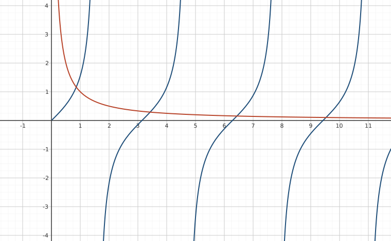
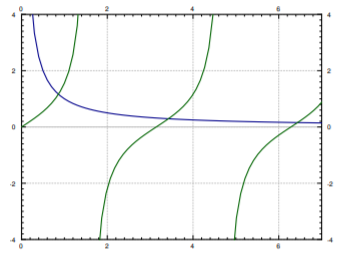
Now use a computer to find $λ_{n}$ . There are tables available, though using a computer or a graphing calculator is far more convenient nowadays. Easiest method is to plot the functions $\frac{h}{x}$ and $\tan (x)$ and see for which they intersect. There is an infinite number of intersections. Denote the first intersection by $the square root of λ sub 1$ the first intersection, by $the square root of λ sub 2$ the second intersection, etc…. For example, when $h equals 1$ , we get that $\sqrt{λ_{1}} \approx 0.86, \sqrt{λ_{2}} \approx 3.43, . . .$ . That is $λ_{1} \approx 0.74, λ_{2} \approx 11.73, . . .$ , …. A plot for $h equals 1$ is given in Figure $1$ . The appropriate eigenfunction (let $A equals 1$ for convenience, then $B = \frac{h}{\sqrt{λ}}$ ) is

Function graph showing y = tan(x) on x in [0.02, 12] and y = h/x on x in [0.02, 12]. Adjustable parameter: Robin constant h (h) = 1. Viewing window: x from -1.79 to 11.79, y from -4.2 to 4.2. — The book's Figure 1 unfrozen. The positive crossings of tan(x) and h/x are the values of √λ, and at h = 1 the first two land on the book's own 0.86 and 3.43. Drag h down toward 0 and every crossing slides toward 0, π, 2π, 3π — the Neumann spectrum, which is exactly the y′(0) = 0, y′(1) = 0 problem this section sets as a Your Turn. Drag it up to 5 and they migrate the other way, toward tan's asymptotes at π/2, 3π/2, 5π/2. At every h the crossings run on forever and each is larger than the last, exactly as the theorem on this page promises.

$y_{n} (x) = \cos (\sqrt{λ_{n}} x) + \frac{h}{\sqrt{λ_{n}}} \sin (\sqrt{λ_{n}} x) .$

When $h equals 1$ we get (approximately)

$y_{1} (x) \approx \cos (0.86 x) + \frac{1}{0.86} \sin (0.86 x), y_{2} (x) \approx \cos (3.43 x) + \frac{1}{3.43} \sin (3.43 x), . . . .$

graph of y = 1/x and y = tan(x) — Figure $1$ : Plot of $\frac{1}{x}$ and $\tan x$ .

Orthogonality

We have seen the notion of orthogonality before. For example, we have shown that $\sin (n x)$ are orthogonal for distinct $n$ on $[ 0, π ]$ . For general Sturm-Liouville problems we will need a more general setup. Let $r (x)$ be a weight function (any function, though generally we will assume it is positive) on $[ a, b ]$ . Two functions $f (x)$ , $g (x)$ are said to be orthogonal with respect to the weight function $r (x)$ when

$∫ a b f open parenthesis x close parenthesis g open parenthesis x close parenthesis r open parenthesis x close parenthesis d x equals 0.$

In this setting, we define the inner product as

$⟨ f, g ⟩ equals d e f ∫ a b f open parenthesis x close parenthesis g open parenthesis x close parenthesis r open parenthesis x close parenthesis d x,$

and then say $f$ and $g$ are orthogonal whenever $⟨ f, g ⟩ equals 0$ . The results and concepts are again analogous to finite dimensional linear algebra.

The idea of the given inner product is that those $x$ where $r (x)$ is greater have more weight. Nontrivial (nonconstant) $r (x)$ arise naturally, for example from a change of variables. Hence, you could think of a change of variables such that $d ξ = r (x) d x$ .

Eigenfunctions of a regular Sturm–Liouville problem satisfy an orthogonality property, just like the eigenfunctions in Section 4.1. Its proof is very similar to the analogous Theorem 4.1.1.

Note

Suppose we have a regular Sturm-Liouville problem

$\begin{matrix} \frac{d}{d x} (p (x) \frac{d y}{d x}) - q (x) y + λ r (x) y = 0, \\ α_{1} y (a) - α_{2} y^{'} (a) = 0, \\ β_{1} y (b) + β_{2} y^{'} (b) = 0 . \end{matrix}$

Let $y_{j}$ and $y_{k}$ be two distinct eigenfunctions for two distinct eigenvalues $λ_{j}$ and $λ_{k}$ . Then

$∫ a b y sub j open parenthesis x close parenthesis y sub k open parenthesis x close parenthesis r open parenthesis x close parenthesis d x equals 0,$

that is, $y_{j}$ and $y_{k}$ are orthogonal with respect to the weight function $r$ .

Fredholm Alternative

We also have the Fredholm alternative theorem we talked about before (Theorem 4.1.2) for all regular Sturm-Liouville problems. We state it here for completeness.

Note

Fredholm Alternative

Suppose that we have a regular Sturm-Liouville problem. Then either

$\begin{matrix} \frac{d}{d x} (p (x) \frac{d y}{d x}) - q (x) y + λ r (x) y = 0, \\ α_{1} y (a) - α_{2} y^{'} (a) = 0, \\ β_{1} y (b) + β_{2} y^{'} (b) = 0, \end{matrix}$

has a nonzero solution, or

$\begin{matrix} \frac{d}{d x} (p (x) \frac{d y}{d x}) - q (x) y + λ r (x) y = f (x), \\ α_{1} y (a) - α_{2} y^{'} (a) = 0, \\ β_{1} y (b) + β_{2} y^{'} (b) = 0, \end{matrix}$

has a unique solution for any $f (x)$ continuous on $[ a, b ]$ .

This theorem is used in much the same way as we did before in Section 4.4. It is used when solving more general nonhomogeneous boundary value problems. The theorem does not help us solve the problem, but it tells us when a unique solution exists, so that we know when to spend time looking for it. To solve the problem we decompose $f (x)$ and $y (x)$ in terms of the eigenfunctions of the homogeneous problem, and then solve for the coefficients of the series for $y (x)$ .

Eigenfunction Series

What we want to do with the eigenfunctions once we have them is to compute the eigenfunction decomposition of an arbitrary function $f (x)$ . That is, we wish to write

$f (x) = \sum_{n = 1}^{\infty} c_{n} y_{n} (x),$

(5.1.2)

where $y_{n} (x)$ the eigenfunctions. We wish to find out if we can represent any function $f (x)$ in this way, and if so, we wish to calculate (and of course we would want to know if the sum converges). OK, so imagine we could write $f (x)$ as (5.1.2). We will assume convergence and the ability to integrate the series term by term. Because of orthogonality we have

$\begin{matrix} ⟨ f, y_{m} ⟩ = \int_{a}^{b} f (x) y_{m} (x) r (x) d x \\ = \sum_{n = 1}^{\infty} c_{n} \int_{a}^{b} y_{n} (x) y_{m} (x) r (x) d x \\ = c_{m} \int_{a}^{b} y_{m} (x) y_{m} (x) r (x) d x = c_{m} ⟨ y_{m}, y_{m} ⟩ . \end{matrix}$

Hence,

$c_{m} = \frac{⟨ f, y_{m} ⟩}{⟨ y_{m}, y_{m} ⟩} = \frac{\int_{a}^{b} f (x) y_{m} (x) r (x) d x}{\int_{a}^{b} (y_{m} (x))^{2} r (x) d x} .$

(5.1.3)

Note that $y_{m}$ are known up to a constant multiple, so we could have picked a scalar multiple of an eigenfunction such that $⟨ y sub m, y sub m ⟩ equals 1$ (if we had an arbitrary eigenfunction ${\tilde{y}}_{m}$ , divide it by $\sqrt{⟨ {\tilde{y}}_{m}, {\tilde{y}}_{m} ⟩}$ ). When $⟨ y sub m, y sub m ⟩ equals 1$ we have the simpler form $c_{m} = ⟨ f, y_{m} ⟩$ as we did for the Fourier series. The following theorem holds more generally, but the statement given is enough for our purposes.

Example 4

Take the simple Sturm-Liouville problem

$\begin{matrix} y^{″} + λ y = 0, 0 < x < \frac{π}{2}, \\ y (0) = 0, y^{'} (\frac{π}{2}) = 0 . \end{matrix}$

The above is a regular problem and furthermore we know by Theorem $1$ that $λ greater than or equal to 0$ .

Suppose $λ equals 0$ , then the general solution is $y (x) A x + B$ , we plug in the initial conditions to get $0 = y (0) = B$ , and $0 = y^{'} (π / 2) = A$ , hence $λ equals 0$ is not an eigenvalue. The general solution, therefore, is

$y (x) = A \cos (\sqrt{λ} x) + B \sin (\sqrt{λ} x) .$

Plugging in the boundary conditions we get $0 = y (0) = A$ and $0 = y^{'} (π / 2) = \sqrt{λ} B \cos (\sqrt{λ} \frac{π}{2})$ . $B$ cannot be zero and hence $\cos (\sqrt{λ} \frac{π}{2} = 0)$ . This means that $\sqrt{λ} \frac{π}{2}$ must be an odd integral multiple of $\frac{π}{2}$ , i.e. $(2 n - 1) \frac{π}{2} = \sqrt{λ_{n}} \frac{π}{2}$ . Hence

$λ_{n} = (2 n - 1)^{2} .$

We can take $B equals 1$ . Hence our eigenfunctions are

$y_{n} (x) = \sin ((2 n - 1) x) .$

Finally we compute

$\int_{0}^{\frac{π}{2}} (\sin ((2 n - 1) x))^{2} d x = \frac{π}{4} .$

So any piecewise smooth function on $[ 0, π / 2 ]$ can be written as

$f (x) = \sum_{n = 1}^{\infty} c_{n} \sin ((2 n - 1) x),$

where

$c_{n} = \frac{⟨ f, y_{n} ⟩}{⟨ y_{n}, y_{n} ⟩} = \frac{\int_{0}^{\frac{π}{2}} \sin ((2 n - 1) x) d x}{\int_{0}^{\frac{π}{2}} (\sin ((2 n - 1) x))^{2} d x} = \frac{4}{π} \int f (x)_{0}^{\frac{π}{2}} \sin ((2 n - 1) x) d x .$

Note that the series converges to an odd $2 π$ -periodic (not $π$ -periodic!) extension of $f (x)$ .

Let us compute an example. Consider $f (x) = x$ for $0 < x < \frac{π}{2}$ . Some calculus later we find

$c_{n} = \frac{4}{π} \int_{0}^{\frac{π}{2}} f (x) \sin ((2 n - 1) x) d x = \frac{4 {(- 1)}^{n + 1}}{π {(2 n - 1)}^{2}},$

and so for

x

[0, \frac{π}{2}]

$f (x) = \sum_{n = 1}^{\infty} \frac{4 {(- 1)}^{n + 1}}{π {(2 n - 1)}^{2}} \sin ((2 n - 1) x) .$

This is different from the $π$ -periodic regular sine series which can be computed to be

$f (x) = \sum_{n = 1}^{\infty} \frac{(- 1)^{n + 1}}{n} \sin (2 n x) .$

Both sums converge are equal to $f (x)$ for $0 < x < \frac{π}{2}$ , but the eigenfunctions involved come from different eigenvalue problems.

Footnotes

[1] Named after the French mathematicians Jacques Charles François Sturm (1803–1855) and Joseph Liouville (1809–1882).

Adapted from Differential Equations for Engineers by Jiří Lebl (Oklahoma State University), hosted on LibreTexts (math.libretexts.org) and licensed under CC BY-SA 4.0. Changes were made. License: CC-BY-SA-4.0.