5.2 Application of Eigenfunction Series

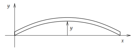
The eigenfunction series can arise even from higher order equations. Consider an elastic beam (say made of steel). We will study the transversal vibrations of the beam. That is, suppose the beam lies along the $x$-axis and let $y(x,t)$ measure the displacement of the point $x$ on the beam at time $t$. See Figure $\PageIndex{1}$.

The equation that governs this setup is

$$a^4 \frac{\partial^4y}{\partial x^4}+\frac{\partial^2y}{\partial t^2}=0, \nonumber$$

for some constant $a>0$, let us not worry about the physics1.

Suppose the beam is of length $1$ simply supported (hinged) at the ends. The beam is displaced by some function $f(x)$ at time $t=0$ and then let go (initial velocity is $0$). Then $y$ satisfies:

Again we try $y(x,t)=X(x)T(t)$ and plug in to get $a^4X^{(4)}T+XT''=0$ or

$$\frac{X^{(4)}}{X}=\frac{-T''}{a^4T}=\lambda. \nonumber$$

The equations are

$$T'' + \lambda a^4 T = 0, \qquad X^{(4)} - \lambda X = 0. \nonumber$$

$$X(0) = X''(0) = 0, \qquad \text{and} \qquad X(1) = X''(1) = 0. \nonumber$$

The initial homogeneous condition $y_t(x,0) = 0$ implies

$$T'(0) = 0. \nonumber$$

Considering the equation for $T$, that is, $T'' + \lambda a^4 T = 0$, and physical intuition leads us to the fact that if $\lambda$ is an eigenvalue then $\lambda > 0$: We expect vibration and not exponential growth nor decay in the $t$ direction (there is no friction in our model for instance). So there are no negative eigenvalues. Similarly $\lambda = 0$ is not an eigenvalue.

Write $\omega^4=\lambda$, so that we do not need to write the fourth root all the time. For $X$ we get the equation $X^{(4)}- \omega^4X=0$. The general solution is

$$X(x)=Ae^{\omega x}+Be^{- \omega x}+C\sin(\omega x)+D\cos(\omega x). \nonumber$$

Now $$0=X(0)A+B+D, 0=X''(0)=\omega^2(A+B-D)$$. Hence, $D=0$ and $A+B=0$, or $B=-A$. So we have

$$X(x)=Ae^{\omega x}-Ae^{- \omega x}+C\sin(\omega x). \nonumber$$

Also $$0=X(1)=A(e^{\omega}-e^{- \omega})+C\sin \omega$$, and $$0=X''(1)=A\omega^2(e^{\omega}-e^{- \omega})-C\omega^2\sin \omega$$. This means that $C\sin \omega =0$ and $A(e^{\omega}-e^{- \omega})=2A\sinh \omega=0$. If $\omega >0$, then $\omega \neq 0$ and so $A=0$. This means that $C \neq 0$ otherwise $\lambda$ is not an eigenvalue. Also $\omega$ must be an integer multiple of $\pi$. Hence $\omega =n\pi$ and $n \geq 1$ (as $\omega >0$). We can take $C=1$. So the eigenvalues are $\lambda_n=n^4\pi^4$ and the eigenfunctions are $\sin(n\pi x)$.

Now $T''+n^4\pi^4a^4T=0$. The general solution is $$T(t)=A\sin(n^2\pi^2a^2t)+B\cos(n^2\pi^2a^2t)$$. But $T'(0)=0$ and hence we must have $A=0$ and we can take $B=1$ to make $T(0)=1$ for convenience. So our solutions are $T_n(t)=\cos(n^2\pi^2a^2t)$.

As the eigenfunctions are just sines again, we can decompose the function $f(x)$ on $0<x<1$ using the sine series. We find numbers $b_n$ such that for $0<x<1$ we have

$$f(x)=\sum_{n=1}^{\infty}b_n\sin(n\pi x). \nonumber$$

Then the solution to (5.2.1) is

$$y(x,t)=\sum_{n=1}^{\infty}b_nX_n(x)T_n(t)=\sum_{n=1}^{\infty}b_n\sin(n\pi x)\cos(n^2\pi^2a^2t). \nonumber$$

The point is that $X_nT_n$ is a solution that satisfies all the homogeneous conditions (that is, all conditions except the initial position). And since and $T_n(0)=1$, we have

$$y(x,0)=\sum_{n=1}^{\infty}b_nX_n(x)T_n(0)=\sum_{n=1}^{\infty}b_nX_n(x)=\sum_{n=1}^{\infty}b_n\sin(n\pi x)=f(x). \nonumber$$

So $y(x,t)$ solves (5.2.1).

The natural (circular) frequencies of the system are $n^2\pi^2a^2$. These frequencies are all integer multiples of the fundamental frequency $\pi^2a^2$, so we get a nice musical note. The exact frequencies and their amplitude are what we call the timbre of the note.

The timbre of a beam is different than for a vibrating string where we get “more” of the lower frequencies since we get all integer multiples, $1,2,3,4,5, \ldots$. For a steel beam we get only the square multiples $1,4,9,16,25, \ldots$. That is why when you hit a steel beam you hear a very pure sound. The sound of a xylophone or vibraphone is, therefore, very different from a guitar or piano.

There are other boundary conditions than just hinged ends. There are three basic possibilities: hinged, free, or fixed. Let us consider the end at $x=0$. For the other end, it is the same idea. If the end is hinged, then

$$u(0,t) = u_{xx}(0,t) = 0. \nonumber$$

$$u_{xx}(0,t) = u_{xxx}(0,t) = 0. \nonumber$$

$$u(0,t) = u_{x}(0,t) = 0. \nonumber$$

Footnotes

[1] If you are interested, $a^{4}=\frac{EI}{\rho}$, where $E$ is the elastic modulus, $I$ is the second moment of area of the cross section, and $\rho$ is linear density.

Adapted from Differential Equations for Engineers by Jiří Lebl (https://www.jirka.org/diffyqs/), © Jiří Lebl, licensed under CC BY-SA 4.0. Changes were made. License: CC-BY-SA-4.0.