13.4 Distributions

13.4.1 Normal changing mean

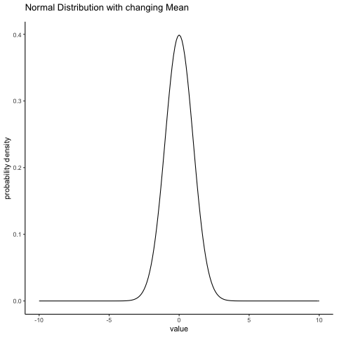
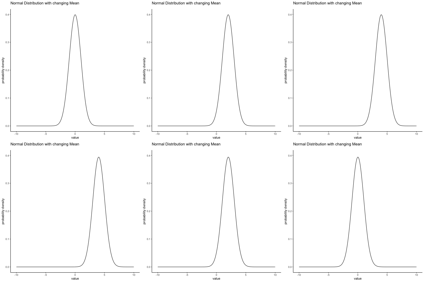
Animation of a normal distribution with a changing mean: a bell curve of constant width and height slides smoothly rightward along the axis as its mean steps from 0 up to 5, then slides back toward 0 and repeats. Only the curve's location shifts; its shape never changes. — View animation (GIF)

Source R listing: this example needs additional R packages not bundled with the browser runtime. The original code is preserved for use in a local R session; it is not a browser Run cell.

some_means<-c(0,1,2,3,4,5,4,3,2,1)
all_df<-data.frame()
for(i in 1:10){
  dnorm_vec <- dnorm(seq(-10,10,.1),mean=some_means[i],sd=1)
  x_range   <- seq(-10,10,.1)
  means <- rep(some_means[i], length(x_range))
  sims <- rep(i, length(x_range))
  t_df<-data.frame(sims,means,x_range,dnorm_vec)
  all_df<-rbind(all_df,t_df)
}

ggplot(all_df, aes(x=x_range,y=dnorm_vec))+
  geom_line()+
  theme_classic()+
  ylab("probability density")+
  xlab("value")+
  ggtitle("Normal Distribution with changing Mean")+
   transition_states(
    sims,
    transition_length = 1,
    state_length = 1
  )
  #enter_fade() + 
  #exit_shrink() +
  #ease_aes('sine-in-out')

13.4.2 Normal changing sd

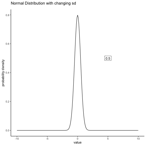
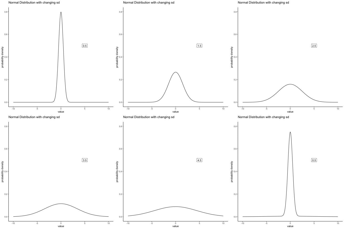
Animation of a normal distribution centered at 0 while its standard deviation changes: the curve begins tall and narrow at SD 0.5, then progressively flattens and spreads out as the SD steps up to 5, and cycles back to narrow again. A label in the plot shows the current SD at each step. — View animation (GIF)

Source R listing: this example needs additional R packages not bundled with the browser runtime. The original code is preserved for use in a local R session; it is not a browser Run cell.

some_sds<-seq(0.5,5,.5)
all_df<-data.frame()
for(i in 1:10){
  dnorm_vec <- dnorm(seq(-10,10,.1),mean=0,sd=some_sds[i])
  x_range   <- seq(-10,10,.1)
  sds <- rep(some_sds[i], length(x_range))
  sims <- rep(i, length(x_range))
  t_df<-data.frame(sims,sds,x_range,dnorm_vec)
  all_df<-rbind(all_df,t_df)
}

labs_df<-data.frame(sims=1:10,
                    sds=as.character(seq(0.5,5,.5)))

ggplot(all_df, aes(x=x_range,y=dnorm_vec, frame=sims))+
  geom_line()+
  theme_classic()+
  ylab("probability density")+
  xlab("value")+
  ggtitle("Normal Distribution with changing sd")+
  geom_label(data = labs_df, aes(x = 5, y = .5, label = sds))+
   transition_states(
    sims,
    transition_length = 2,
    state_length = 1
  )+
  enter_fade() + 
  exit_shrink() +
  ease_aes('sine-in-out')

Adapted from Answering Questions with Data: Introductory Statistics for Psychology Students, by Matthew J. C. Crump (Brooklyn College of CUNY), crumplab.com/statistics, licensed under CC BY-SA 4.0. Portions adapt Danielle Navarro's Learning Statistics with R (CC BY-SA). Changes were made; this adaptation is distributed under the same license. License: CC-BY-SA-4.0.