Point charges, such as electrons, are among the fundamental building blocks of matter. Furthermore, spherical charge distributions (such as charge on a metal sphere) create external electric fields exactly like a point charge. The electric potential due to a point charge is, thus, a case we need to consider.
We can use calculus to find the work needed to move a test charge q from a large distance away to a distance of r from a point charge q. Noting the connection between work and potential as in the last section, we can obtain the following result.
The potential at infinity is chosen to be zero. Thus, V for a point charge decreases with distance, whereas for a point charge decreases with distance squared:
Recall that the electric potential difference V is a scalar and has no direction, whereas the electric field is a vector. To find the voltage due to a combination of point charges, given zero voltage at infinitely far away, you add the individual voltages as numbers. We will assume for the rest of this chapter that there is zero voltage measured infinitely far away. To find the total electric field, you must add the individual fields as vectors, taking magnitude and direction into account. This is consistent with the fact that V is closely associated with energy, a scalar, whereas is closely associated with force, a vector.
The voltages in both of these examples could be measured with a meter that compares the measured potential with ground potential. Ground potential is often taken to be zero (instead of taking the potential at infinity to be zero). It is the potential difference between two points that is of importance, and very often there is a tacit assumption that some reference point, such as Earth or a very distant point, is at zero potential. As noted earlier, this is analogous to taking sea level as when considering gravitational potential energy .
Systems of Multiple Point Charges
Just as the electric field obeys a superposition principle, so does the electric potential. Consider a system consisting of N charges What is the net electric potential V at a space point P from these charges? Each of these charges is a source charge that produces its own electric potential at point P, independent of whatever other changes may be doing. Let be the electric potentials at P produced by the charges respectively. Then, the net electric potential at that point is equal to the sum of these individual electric potentials. You can easily show this by calculating the potential energy of a test charge when you bring the test charge from the reference point at infinity to point P:
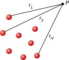
Note that electric potential follows the same principle of superposition as electric field and electric potential energy. To show this more explicitly, note that a test charge at the point P in space has distances of from the N charges fixed in space above, as shown in Figure 7.19. Using our formula for the potential of a point charge for each of these (assumed to be point) charges, we find that
(7.9)
Therefore, the electric potential energy of the test charge is
which is the same as the work to bring the test charge into the system, as found in the first section of the chapter.
Figure 7.19Notation for direct distances from charges to a space point P.
The Electric Dipole
An electric dipole is a system of two equal but opposite charges a fixed distance apart. This system is used to model many real-world systems, including atomic and molecular interactions. One of these systems is the water molecule, under certain circumstances. These circumstances are met inside a microwave oven, where electric fields with alternating directions make the water molecules change orientation. This vibration is the same as heat at the molecular level.
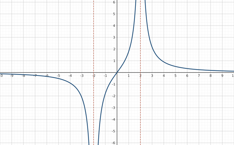
Interactive figureElectric potential along the axis of a dipole, with the separation on a sliderDrag the Charge separation d (the worked example uses 4.0 cm) slider from 0.5 to 8.
XYZ Graph · viewer build 5edf91b
The example Electric Potential of a Dipole, seen along the dipole's own axis: charges of q = 3.0 nC and −3.0 nC separated by d = 4.0 cm, with V = kΣqᵢ/rᵢ = 2.70(1/|z − d/2| − 1/|z + d/2|). The horizontal axis is z in centimetres and the vertical axis is the potential in kilovolts; the two dashed vertical lines sit on the charges and move with the slider. The example's own answers are points on this curve — at z = 1.0 cm it reads 1.8 kV and at z = −5.0 cm it reads −0.51 kV, both matching the book to the digits given. Between the charges the curve is steep and one-signed; outside them it collapses toward zero from both ends, and it crosses zero exactly at the midpoint, which is the Check Your Understanding answer that the potential vanishes on the plane bisecting the dipole. Now close the separation with the slider. The two spikes march together and the far field dies away faster and faster: at large z the two 1/r terms cancel to leading order and what is left is the dipole potential kp cos θ/r², falling as 1/z² rather than 1/z.
Now let us consider the special case when the distance of the point P from the dipole is much greater than the distance between the charges in the dipole, for example, when we are interested in the electric potential due to a polarized molecule such as a water molecule. This is not so far (infinity) that we can simply treat the potential as zero, but the distance is great enough that we can simplify our calculations relative to the previous example.
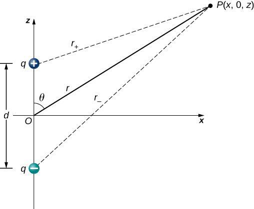
We start by noting that in Figure 7.21 the potential is given by
where
Figure 7.21A general diagram of an electric dipole, and the notation for the distances from the individual charges to a point P in space.
This is still the exact formula. To take advantage of the fact that we rewrite the radii in terms of polar coordinates, with and . This gives us
We can simplify this expression by pulling r out of the root,
and then multiplying out the parentheses
The last term in the root is small enough to be negligible (remember and hence is extremely small, effectively zero to the level we will probably be measuring), leaving us with
Using the binomial approximation (a standard result from the mathematics of series, when is small)
and substituting this into our formula for , we get
This may be written more conveniently if we define a new quantity, the electric dipole moment,
where these vectors point from the negative to the positive charge. Note that this has magnitude qd. This quantity allows us to write the potential at point P due to a dipole at the origin as
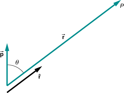
A diagram of the application of this formula is shown in Figure 7.22.
Figure 7.22The geometry for the application of the potential of a dipole.
There are also higher-order moments, for quadrupoles, octupoles, and so on. You will see these in future classes.
Potential of Continuous Charge Distributions
We have been working with point charges a great deal, but what about continuous charge distributions? Recall from Equation 7.9 that
We may treat a continuous charge distribution as a collection of infinitesimally separated individual points. This yields the integral
for the potential at a point P. Note that r is the distance from each individual point in the charge distribution to the point P. As we saw in Electric Charges and Fields, the infinitesimal charges are given by
where is linear charge density, is the charge per unit area, and is the charge per unit volume.
Summary
Electric potential is a scalar whereas electric field is a vector.
Addition of voltages as numbers gives the voltage due to a combination of point charges, allowing us to use the principle of superposition: .
An electric dipole consists of two equal and opposite charges a fixed distance apart, with a dipole moment .
Continuous charge distributions may be calculated with .
Conceptual Questions
Compare the electric dipole moments of charges separated by a distance d and charges separated by a distance d/2.
The second has 1/4 the dipole moment of the first.
Would Gauss’s law be helpful for determining the electric field of a dipole? Why?
In what region of space is the potential due to a uniformly charged sphere the same as that of a point charge? In what region does it differ from that of a point charge?
The region outside of the sphere will have a potential indistinguishable from a point charge; the interior of the sphere will have a different potential.
Can the potential of a nonuniformly charged sphere be the same as that of a point charge? Explain.
Problems
A 0.500-cm-diameter plastic sphere, used in a static electricity demonstration, has a uniformly distributed 40.0-pC charge on its surface. What is the potential near its surface?
How far from a point charge is the potential 100 V? At what distance is it
If the potential due to a point charge is at a distance of 15.0 m, what are the sign and magnitude of the charge?
;
The charge is positive because the potential is positive.
In nuclear fission, a nucleus splits roughly in half. (a) What is the potential from a fragment that has 46 protons in it? (b) What is the potential energy in MeV of a similarly charged fragment at this distance?
A research Van de Graaff generator has a 2.00-m-diameter metal sphere with a charge of 5.00 mC on it. Assume the potential energy is zero at a reference point infinitely far away from the Van de Graaff. (a) What is the potential near its surface? (b) At what distance from its center is the potential 1.00 MV? (c) An oxygen atom with three missing electrons is released near the Van de Graaff generator. What is its kinetic energy in MeV when the atom is at the distance found in part b?
a. ;
b. ;
c.
An electrostatic paint sprayer has a 0.200-m-diameter metal sphere at a potential of 25.0 kV that repels paint droplets onto a grounded object.
(a) What charge is on the sphere? (b) What charge must a 0.100-mg drop of paint have to arrive at the object with a speed of 10.0 m/s?
(a) What is the potential between two points situated 10 cm and 20 cm from a point charge? (b) To what location should the point at 20 cm be moved to increase this potential difference by a factor of two?
; a. Relative to origin, find the potential at each point and then calculate the difference.
;
b. To double the potential difference, move the point from 20 cm to infinity; the potential at 20 cm is halfway between zero and that at 10 cm.
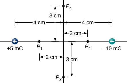
Find the potential at points in the diagram due to the two given charges.
Two charges are separated by 4.0 cm on the z-axis symmetrically about origin, with the positive one uppermost. Two space points of interest are located 3.0 cm and 30 cm from origin at an angle with respect to the z-axis. Evaluate electric potentials at in two ways: (a) Using the exact formula for point charges, and (b) using the approximate dipole potential formula.
a.
and ;
b. and
(a) Plot the potential of a uniformly charged 1-m rod with 1 C/m charge as a function of the perpendicular distance from the center. Draw your graph from . (b) On the same graph, plot the potential of a point charge with a 1-C charge at the origin. (c) Which potential is stronger near the rod? (d) What happens to the difference as the distance increases? Interpret your result.
Adapted from University Physics Volume 2 by OpenStax (openstax.org), licensed under CC BY-NC-SA 4.0. Changes were made. License: CC-BY-NC-SA-4.0.
These eBooks are a prerelease and are not yet certified conformant with WCAG 2.1 AA or ADA Title II. Every page is built against an automated accessibility gate, and the published editions will meet ADA Title II requirements when they release in late September 2026. If something is unusable, please tell us.