3.3 Average and Instantaneous Acceleration

The importance of understanding acceleration spans our day-to-day experience, as well as the vast reaches of outer space and the tiny world of subatomic physics. In everyday conversation, to accelerate means to speed up; applying the brake pedal causes a vehicle to slow down. We are familiar with the acceleration of our car, for example. The greater the acceleration, the greater the change in velocity over a given time. Acceleration is widely seen in experimental physics. In linear particle accelerator experiments, for example, subatomic particles are accelerated to very high velocities in collision experiments, which tell us information about the structure of the subatomic world as well as the origin of the universe. In space, cosmic rays are subatomic particles that have been accelerated to very high energies in supernovas (exploding massive stars) and active galactic nuclei. It is important to understand the processes that accelerate cosmic rays because these rays contain highly penetrating radiation that can damage electronics flown on spacecraft, for example.

Average Acceleration

The formal definition of acceleration is consistent with these notions just described, but is more inclusive.

Because acceleration is velocity in meters per second divided by time in seconds, the SI units for acceleration are often abbreviated m/s²—that is, meters per second squared or meters per second per second. This literally means by how many meters per second the velocity changes every second. Recall that velocity is a vector—it has both magnitude and direction—which means that a change in velocity can be a change in magnitude (or speed), but it can also be a change in direction. For example, if a runner traveling at 10 km/h due east slows to a stop, reverses direction, and continues her run at 10 km/h due west, her velocity has changed as a result of the change in direction, although the magnitude of the velocity is the same in both directions. Thus, acceleration occurs when velocity changes in magnitude (an increase or decrease in speed) or in direction, or both.

Keep in mind that although acceleration is in the direction of the change in velocity, it is not always in the direction of motion. When an object slows down, its acceleration is opposite to the direction of its motion. Although this is commonly referred to as deceleration Figure 3.10, we say the train is accelerating in a direction opposite to its direction of motion.

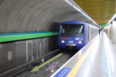
Picture shows a subway train coming into a station. — **Figure 3.10** A subway train in Sao Paulo, Brazil, accelerates opposite to the motion as it comes into a station. It is accelerating in a direction opposite to its direction of motion.A subway train in Sao Paulo, Brazil, accelerates opposite to the motion as it comes into a station. It is accelerating in a direction opposite to its direction of motion. (credit: modification of work by Yusuke Kawasaki)

The term deceleration can cause confusion in our analysis because it is not a vector and it does not point to a specific direction with respect to a coordinate system, so we do not use it. Acceleration is a vector, so we must choose the appropriate sign for it in our chosen coordinate system. In the case of the train in Figure 3.10, acceleration is in the negative direction in the chosen coordinate system, so we say the train is undergoing negative acceleration.

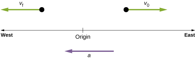
If an object in motion has a velocity in the positive direction with respect to a chosen origin and it acquires a constant negative acceleration, the object eventually comes to a rest and reverses direction. If we wait long enough, the object passes through the origin going in the opposite direction. This is illustrated in Figure 3.11.

Figure shows three vectors: a directed to the west, vf directed to the west, and vo directed to the east. — **Figure 3.11** An object in motion with a velocity vector toward the east under negative acceleration comes to a rest and reverses direction. It passes the origin going in the opposite direction after a long enough time.

Example 1 Calculating Average Acceleration: A Racehorse Leaves the Gate

A racehorse coming out of the gate accelerates from rest to a velocity of 15.0 m/s due west in 1.80 s. What is its average acceleration?

Figure 3.12 Racehorses accelerating out of the gate.Racehorses accelerating out of the gate. (credit: modification of work by Jon Sullivan)

Strategy First we draw a sketch and assign a coordinate system to the problem Figure 3.13. This is a simple problem, but it always helps to visualize it. Notice that we assign east as positive and west as negative. Thus, in this case, we have negative velocity.

Figure 3.13 Identify the coordinate system, the given information, and what you want to determine.

We can solve this problem by identifying $Δ v and Δ t$ from the given information, and then calculating the average acceleration directly from the equation $\overset{–}{a} = \frac{Δ v}{Δ t} = \frac{v_{f} - v_{0}}{t_{f} - t_{0}}$ .

Solution First, identify the knowns: $v_{0} = 0, v_{f} = −15.0 m/s$ (the negative sign indicates direction toward the west), Δt = 1.80 s.

Second, find the change in velocity. Since the horse is going from zero to –15.0 m/s, its change in velocity equals its final velocity:

$Δ v = v_{f} - v_{0} = v_{f} = −15.0 m/s .$

Last, substitute the known values ( $Δ v and Δ t$ ) and solve for the unknown $\overset{–}{a}$ :

$\overset{–}{a} = \frac{Δ v}{Δ t} = \frac{−15.0 m/s}{1.80 s} = −8.33 {m/s}^{2} .$

Significance The negative sign for acceleration indicates that acceleration is toward the west. An acceleration of 8.33 m/s² due west means the horse increases its velocity by 8.33 m/s due west each second; that is, 8.33 meters per second per second, which we write as 8.33 m/s². This is truly an average acceleration, because the ride is not smooth. We see later that an acceleration of this magnitude would require the rider to hang on with a force nearly equal to his weight.

Instantaneous Acceleration

Instantaneous acceleration a, or acceleration at a specific instant in time, is obtained using the same process discussed for instantaneous velocity. That is, we calculate the average acceleration between two points in time separated by $Δ t$ and let $Δ t$ approach zero. The result is the derivative of the velocity function v(t), which is instantaneous acceleration and is expressed mathematically as

$a (t) = \frac{d}{d t} v (t) .$

(3.9)

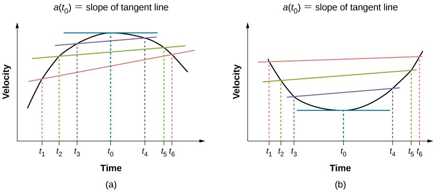
Thus, similar to velocity being the derivative of the position function, instantaneous acceleration is the derivative of the velocity function. We can show this graphically in the same way as instantaneous velocity. In Figure 3.14, instantaneous acceleration at time t₀ is the slope of the tangent line to the velocity-versus-time graph at time t₀. We see that average acceleration $\overset{–}{a} = \frac{Δ v}{Δ t}$ approaches instantaneous acceleration as $Δ t$ approaches zero. Also in part (a) of the figure, we see that velocity has a maximum when its slope is zero. This time corresponds to the zero of the acceleration function. In part (b), instantaneous acceleration at the minimum velocity is shown, which is also zero, since the slope of the curve is zero there, too. Thus, for a given velocity function, the zeros of the acceleration function give either the minimum or the maximum velocity.

Graph A shows velocity plotted versus time. Velocity increases from t1 to t2 and t3. It reaches maximum at t0. It decreases to t4 and continues to decrease to t5 and t6. The slope of the tangent line at t0 is indicated as the instantaneous velocity. Graph B shows velocity plotted versus time. Velocity decreases from t1 to t2 and t3. It reaches minimum at t0. It increases to t4 and continues to increase to t5 and t6. The slope of the tangent line at t0 is indicated as the instantaneous velocity. — **Figure 3.14** In a graph of velocity versus time, instantaneous acceleration is the slope of the tangent line. (a) Shown is average acceleration $\overset{–}{a} = \frac{Δ v}{Δ t} = \frac{v_{f} - v_{i}}{t_{f} - t_{i}}$ between times $Δ t = t_{6} - t_{1}, Δ t = t_{5} - t_{2}$ , and $Δ t = t_{4} - t_{3}$ . When $Δ t → 0$ , the average acceleration approaches instantaneous acceleration at time t₀. In view (a), instantaneous acceleration is shown for the point on the velocity curve at maximum velocity. At this point, instantaneous acceleration is the slope of the tangent line, which is zero. At any other time, the slope of the tangent line—and thus instantaneous acceleration—would not be zero. (b) Same as (a) but shown for instantaneous acceleration at minimum velocity.

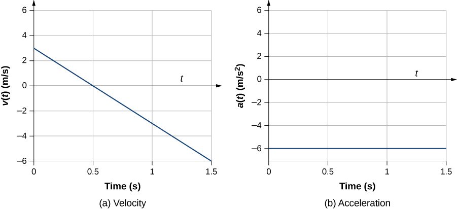
To illustrate this concept, let’s look at two examples. First, a simple example is shown using Figure 3.9(b), the velocity-versus-time graph of Example 3 in Section 3.2, to find acceleration graphically. This graph is depicted in Figure 3.15(a), which is a straight line. The corresponding graph of acceleration versus time is found from the slope of velocity and is shown in Figure 3.15(b). In this example, the velocity function is a straight line with a constant slope, thus acceleration is a constant. In the next example, the velocity function has a more complicated functional dependence on time.

Graph A shows velocity in meters per second plotted versus time in seconds. Graph is linear and has a negative constant slope. Graph B shows acceleration in meters per second square plotted versus time in seconds. Graph is linear and has a zero slope with the acceleration being equal to -6. — **Figure 3.15** (a, b) The velocity-versus-time graph is linear and has a negative constant slope (a) that is equal to acceleration, shown in (b).

If we know the functional form of velocity, v(t), we can calculate instantaneous acceleration a(t) at any time point in the motion using Equation 3.9.

Example 2 Calculating Instantaneous Acceleration

A particle is in motion and is accelerating. The functional form of the velocity is $v (t) = (20 {m/s}^{2}) t - (5 {m/s}^{3}) t^{2}$ .

Find the functional form of the acceleration.
Find the instantaneous velocity at t = 1, 2, 3, and 5 s.
Find the instantaneous acceleration at t = 1, 2, 3, and 5 s.
Interpret the results of (c) in terms of the directions of the acceleration and velocity vectors.

Strategy We find the functional form of acceleration by taking the derivative of the velocity function. Then, we calculate the values of instantaneous velocity and acceleration from the given functions for each. For part (d), we need to compare the directions of velocity and acceleration at each time.

Solution

$a (t) = \frac{d v (t)}{d t} = (20 {m/s}^{2}) - (10 {m/s}^{3}) t$
$v open parenthesis 1 s close parenthesis equals 15 m/s$ , $v open parenthesis 2 s close parenthesis equals 20 m/s$ , $v open parenthesis 3 s close parenthesis equals 15 m/s$ , $v open parenthesis 5 s close parenthesis equals −25 m/s$
$a open parenthesis 1 s close parenthesis equals 10 m/s squared$ , $a open parenthesis 2 s close parenthesis equals 0 m/s squared$ , $a open parenthesis 3 s close parenthesis equals −10 m/s squared$ , $a open parenthesis 5 s close parenthesis equals −30 m/s squared$
At t = 1 s, velocity $v open parenthesis 1 s) equals 15 m/s$ is positive and acceleration is positive, so both velocity and acceleration are in the same direction. The particle is moving faster.

At t = 2 s, velocity has increased to $v open parenthesis 2 s) equals 20 m/s$ , where it is maximum, which corresponds to the time when the acceleration is zero. We see that the maximum velocity occurs when the slope of the velocity function is zero, which is just the zero of the acceleration function.

At t = 3 s, velocity is $v open parenthesis 3 s) equals 15 m/s$ and acceleration is negative. The particle has reduced its velocity and the acceleration vector is negative. The particle is slowing down.

At t = 5 s, velocity is $v open parenthesis 5 s) equals −25 m/s$ and acceleration is increasingly negative. Between the times t = 3 s and t = 5 s the particle has decreased its velocity to zero and then become negative, thus reversing its direction. The particle is now speeding up again, but in the opposite direction.

We can see these results graphically in Figure 3.16.

Figure 3.16 (a) Velocity versus time. Tangent lines are indicated at times 1, 2, and 3 s. The slopes of the tangent lines are the accelerations. At t = 3 s, velocity is positive. At t = 5 s, velocity is negative, indicating the particle has reversed direction. (b) Acceleration versus time. Comparing the values of accelerations given by the black dots with the corresponding slopes of the tangent lines (slopes of lines through black dots) in (a), we see they are identical.

Significance By doing both a numerical and graphical analysis of velocity and acceleration of the particle, we can learn much about its motion. The numerical analysis complements the graphical analysis in giving a total view of the motion. The zero of the acceleration function corresponds to the maximum of the velocity in this example. Also in this example, when acceleration is positive and in the same direction as velocity, velocity increases. As acceleration tends toward zero, eventually becoming negative, the velocity reaches a maximum, after which it starts decreasing. If we wait long enough, velocity also becomes negative, indicating a reversal of direction. A real-world example of this type of motion is a car with a velocity that is increasing to a maximum, after which it starts slowing down, comes to a stop, then reverses direction.

Getting a Feel for Acceleration

You are probably used to experiencing acceleration when you step into an elevator, or step on the gas pedal in your car. However, acceleration is happening to many other objects in our universe with which we don’t have direct contact. Table 3.2 presents the acceleration of various objects. We can see the magnitudes of the accelerations extend over many orders of magnitude.

**Table 3.2** Typical Values of Acceleration
Acceleration	Value (m/s²)
High-speed train	0.25
Elevator	2
Cheetah	5
Object in a free fall without air resistance near the surface of Earth	9.8
Space shuttle maximum during launch	29
Parachutist peak during normal opening of parachute	59
F16 aircraft pulling out of a dive	79
Explosive seat ejection from aircraft	147
Sprint missile	982
Fastest rocket sled peak acceleration	1540
Jumping flea	3200
Baseball struck by a bat	30,000
Closing jaws of a trap-jaw ant	1,000,000
Proton in the large Hadron collider	$1.9 \times 10^{9}$

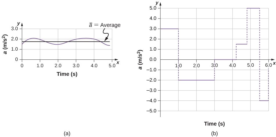
In this table, we see that typical accelerations vary widely with different objects and have nothing to do with object size or how massive it is. Acceleration can also vary widely with time during the motion of an object. A drag racer has a large acceleration just after its start, but then it tapers off as the vehicle reaches a constant velocity. Its average acceleration can be quite different from its instantaneous acceleration at a particular time during its motion. Figure 3.17 compares graphically average acceleration with instantaneous acceleration for two very different motions.

Graph A shows acceleration in meters per second squared plotted versus time in seconds. Acceleration varies only slightly and is always in the same direction, since it is positive. The average over the interval is nearly the same as the acceleration at any given time. Graph B shows acceleration in meters per second squared plotted versus time in seconds. Acceleration varies greatly: from -4 meters per second squared to 5 meters per second squared. — **Figure 3.17** Graphs of instantaneous acceleration versus time for two different one-dimensional motions. (a) Acceleration varies only slightly and is always in the same direction, since it is positive. The average over the interval is nearly the same as the acceleration at any given time. (b) Acceleration varies greatly, perhaps representing a package on a post office conveyor belt that is accelerated forward and backward as it bumps along. It is necessary to consider small time intervals (such as from 0–1.0 s) with constant or nearly constant acceleration in such a situation.

Summary

Acceleration is the rate at which velocity changes. The SI unit for acceleration is meters per second squared.
Acceleration is a vector. It has both magnitude and direction and so can be the rate of change of the magnitude or direction of the velocity, or both.
Instantaneous acceleration a(t) is a continuous function of time and gives the acceleration at any specific time during the motion. It is calculated from the derivative of the velocity function. Instantaneous acceleration is the slope of the velocity-versus-time graph.
Negative acceleration (sometimes called deceleration) is acceleration in the negative direction in the chosen coordinate system.

Conceptual Questions

Is it possible for speed to be constant while acceleration is not zero?

No, in one dimension constant speed requires zero acceleration.

Is it possible for velocity to be constant while acceleration is not zero? Explain.

Give an example in which velocity is zero yet acceleration is not.

A ball is thrown into the air and its velocity is zero at the apex of the throw, but acceleration is not zero.

If a subway train is moving to the left (has a negative velocity) and then comes to a stop, what is the direction of its acceleration? Is the acceleration positive or negative?

Plus and minus signs are used in one-dimensional motion to indicate direction. What is the sign of an acceleration that reduces the magnitude of a negative velocity? Of a positive velocity?

Plus, minus

A cheetah can accelerate from rest to a speed of 30.0 m/s in 7.00 s. What is its acceleration?

$a equals 4.29 m/s squared$

Dr. John Paul Stapp was a U.S. Air Force officer who studied the effects of extreme acceleration on the human body. On December 10, 1954, Stapp rode a rocket sled, accelerating from rest to a top speed of 282 m/s (1015 km/h) in 5.00 s and was brought jarringly back to rest in only 1.40 s. Calculate his (a) acceleration in his direction of motion and (b) acceleration opposite to his direction of motion. Express each in multiples of g (9.80 m/s²) by taking its ratio to the acceleration of gravity.

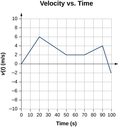
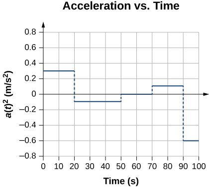
Sketch the acceleration-versus-time graph from the following velocity-versus-time graph.

Graph shows velocity in meters per second plotted versus time in seconds. Velocity is zero and zero seconds, increases to 6 meters per second at 20 seconds, decreases to 2 meters per second at 50 and remains constant until 70 seconds, increases to 4 meters per second at 90 seconds, and decreases to –2 meters per second at 100 seconds.

Graph shows acceleration in meters per second squared plotted versus time in seconds. Acceleration is 0.3 meters per second squared between 0 and 20 seconds, -0.1 meters per second squared between 20 and 50 seconds, zero between 50 and 70 seconds, -0.6 between 90 and 100 seconds.

A commuter backs her car out of her garage with an acceleration of 1.40 m/s². (a) How long does it take her to reach a speed of 2.00 m/s? (b) If she then brakes to a stop in 0.800 s, what is her acceleration?

Assume an intercontinental ballistic missile goes from rest to a suborbital speed of 6.50 km/s in 60.0 s (the actual speed and time are classified). What is its average acceleration in meters per second squared and in multiples of g (9.80 m/s²)?

$a equals 11.1 g$

An airplane, starting from rest, moves down the runway at constant acceleration for 18 s and then takes off at a speed of 60 m/s. What is the average acceleration of the plane?