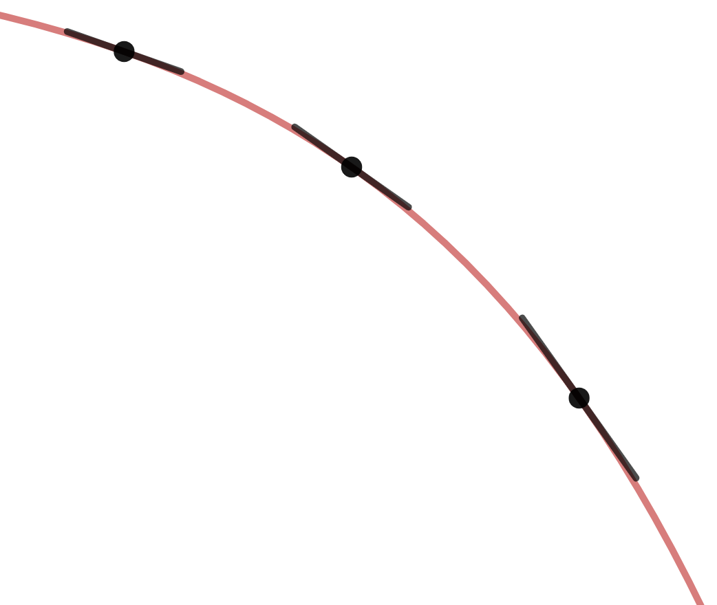
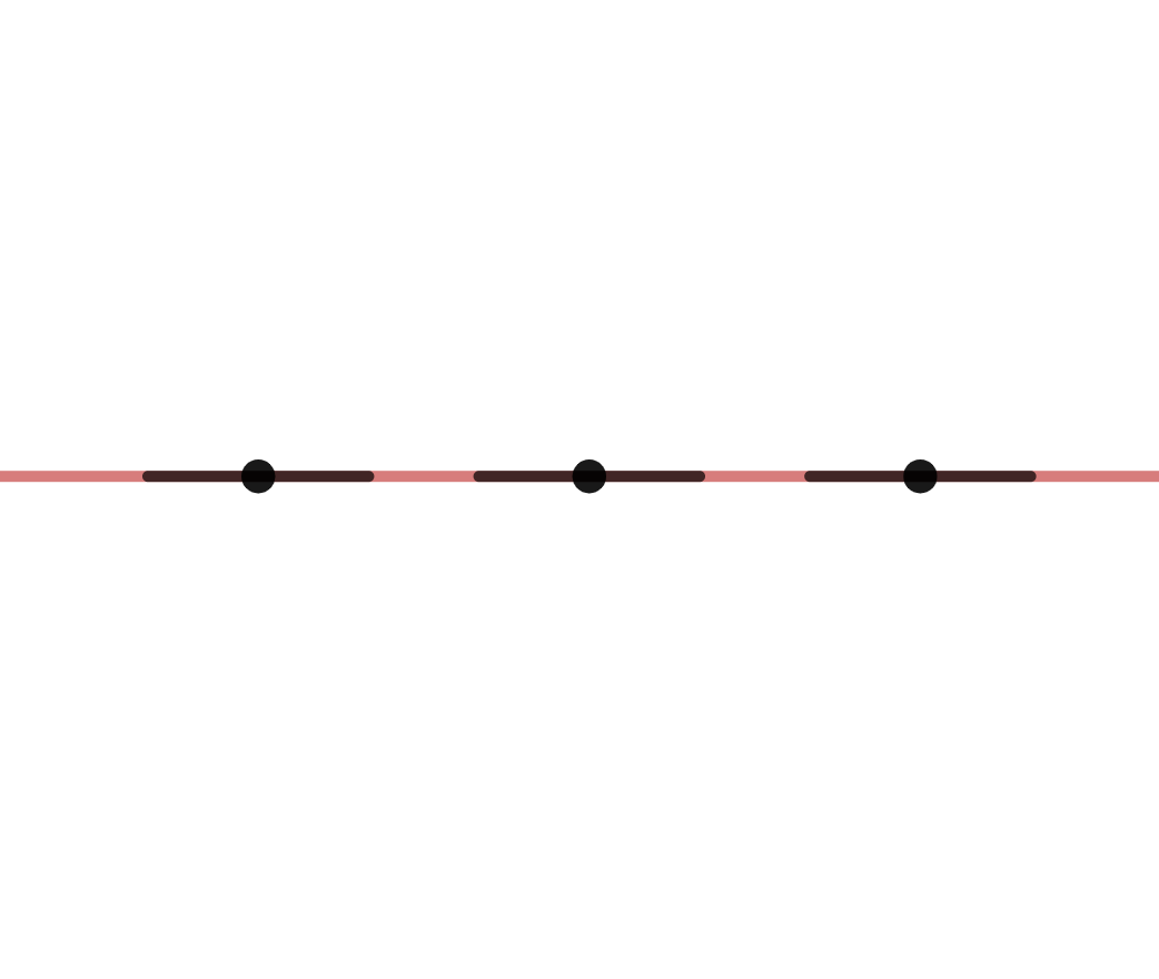
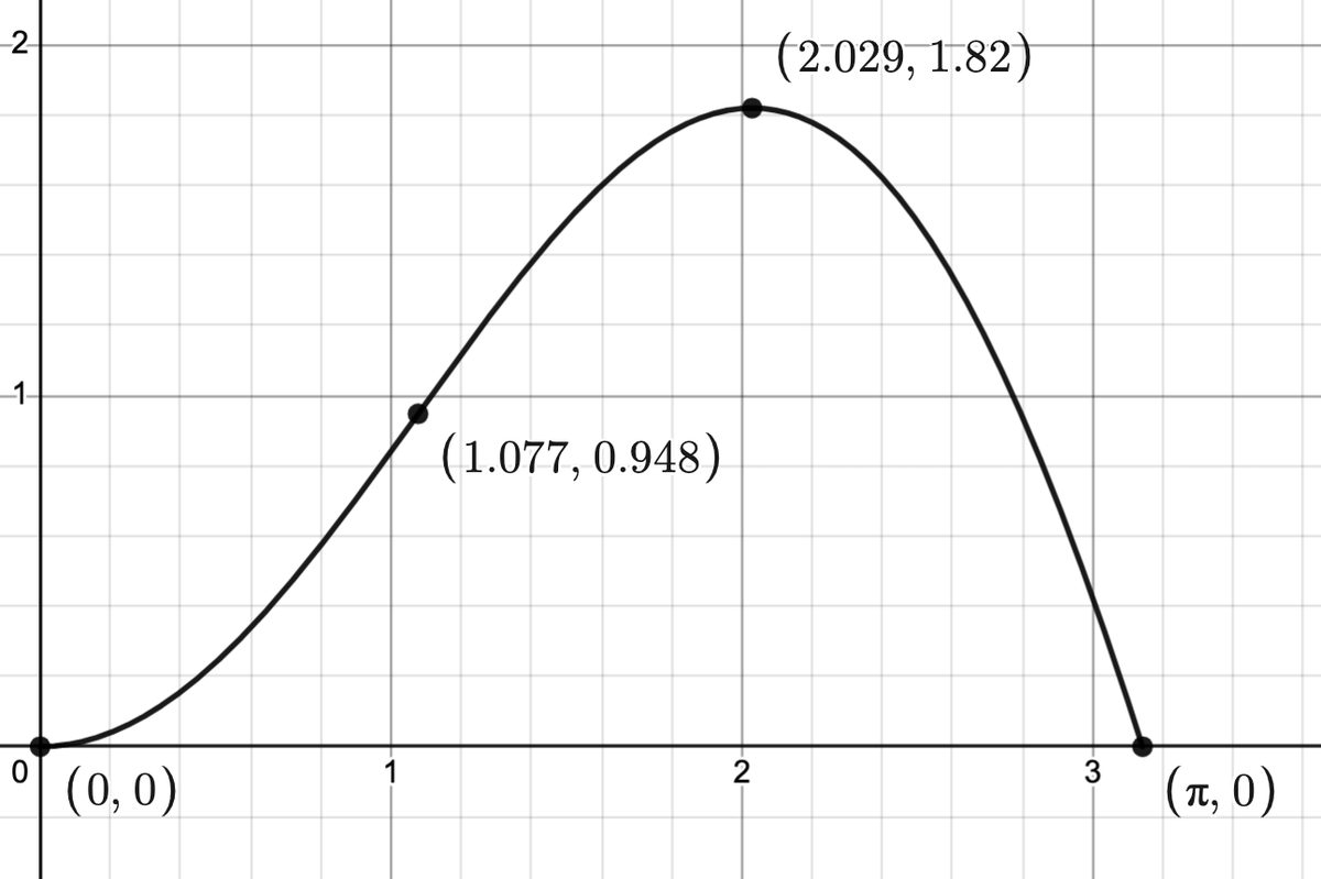
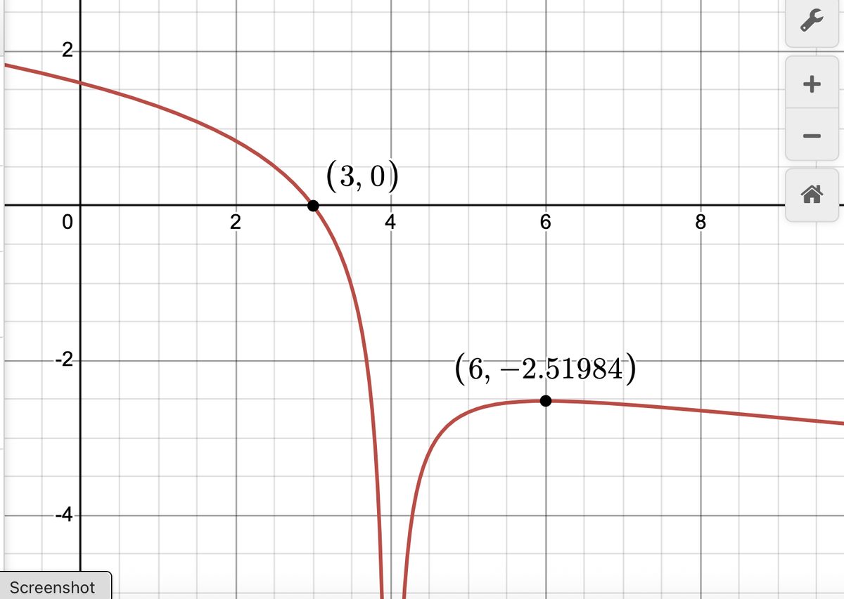
We know if is differentiable at then the graph of is locally linear at and is the slope of the tangent line at the point . In this section, we explore how local behavior near a point can be extrapolated to global behavior over an interval. First, we review Definition 1.7 from Section 1.2:
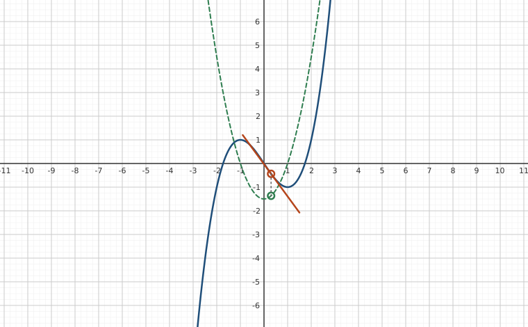
Interactive figureWhere f′ is above the axis, f is climbing: one point, two graphsDrag the Point a slider from -2.5 to 2.5.
XYZ Graph · viewer build 5edf91b
The solid curve is f(x) = (x³ − 3x)/2 and the dashed green curve is its derivative f′(x) = (3x² − 3)/2. A slider moves a point along f; the short rust segment through it is the tangent there, and the green marker directly above or below it on f′ reports the tangent's slope as a height. Wherever the green marker sits above the x-axis the tangent tilts upward and f is increasing; where it dips below, f is decreasing; and at the two points where f′ crosses zero the tangent goes flat at the local maximum and minimum of f.
Suppose a function satisfies for all in an open interval1
. Then we know that not only is the graph of locally linear on , but the slopes of all of the tangent lines are positive. This means that all of the tangent lines are increasing so it stands to reason that the function is likewise increasing on . In other words, if a function is locally increasing on , then it is globally increasing on as well.
We can apply the same reasoning above to situations where for all in , which implies is decreasing on or on , which implies is constant on . In Calculus, you'll learn this fact is a consequence of the Mean Value Theorem.2 In this text, we'll just accept the following theorem is true and hope we've done enough hand-waving to deem it reasonable.
Theorem 6.4 may be visualized as follows:
for all in :
Figure 6.50Figure 6.51
for all in :
Figure 6.52Figure 6.53
for all in :
Figure 6.54
We can use Theorem 6.4 to help us determine the (open) intervals over which a function is increasing, decreasing, and constant by making a sign diagram for the derivative .
In order to avoid us having to go through the (somewhat lengthy) process of finding using Definition 6.8, we'll just use some properties of derivatives from Calculus behind the scenes and present you with both a function and its derivative. It's time for an example.
We generalize our observations about local extrema in the following result.
Concavity and the Second Derivative
In section Section 4.2, we introduced the notion of concavity. In that section, we described curves as being concave up over an interval if it resembles a portion of a `' shape and concave down over an interval if resembles part of a `' shape. Now that we've had some exposure to Calculus, we can more precisely define these notions.
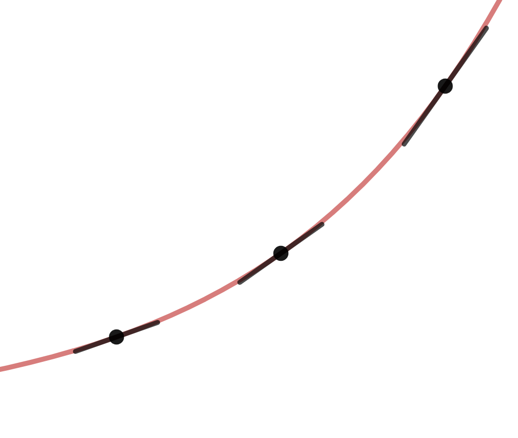
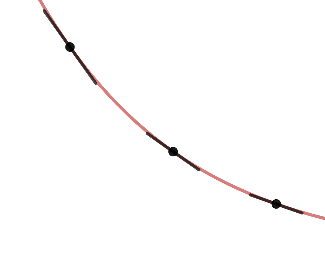
If we take the time to study a generic concave up curve, the `' shape can be divided into a decreasing and increasing arc:
Figure 6.61Figure 6.62
slopes are increasing towards
slopes are increasing away from
In both of these cases, the slopes of the tangent line are increasing.
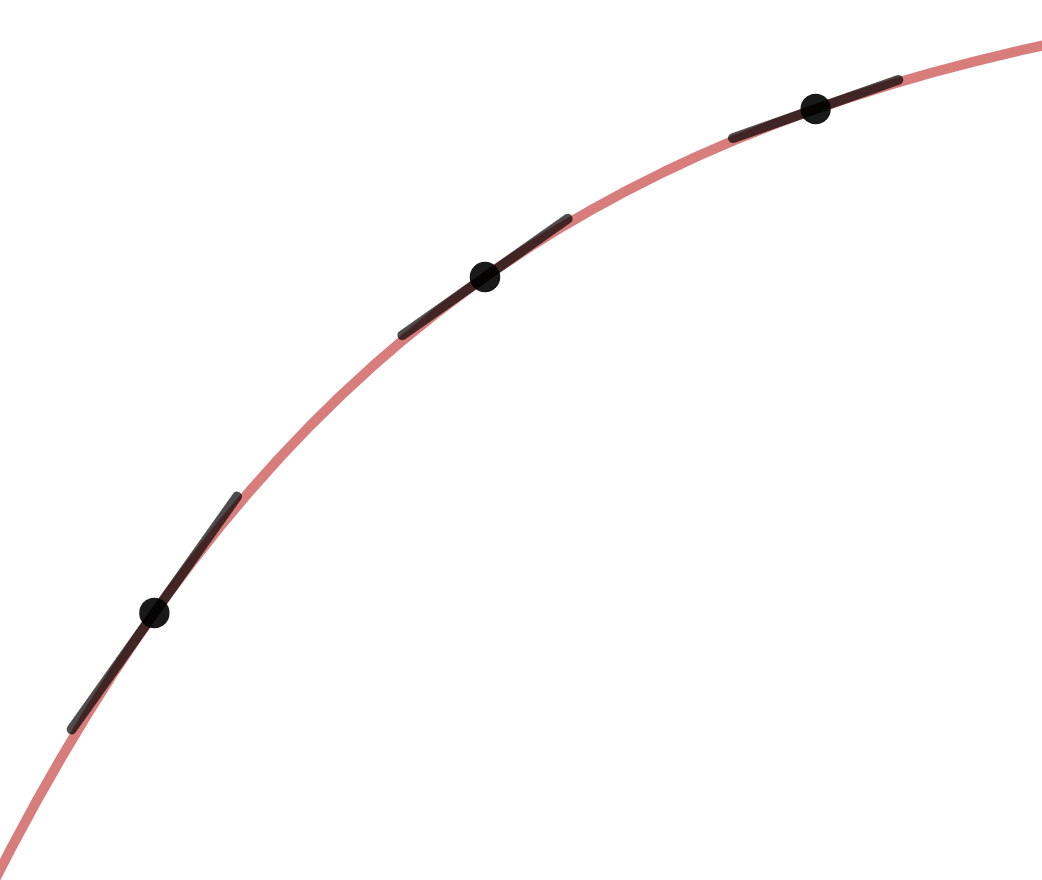
Likewise, we can dissect a generic `' shape curve into an increasing and decreasing arc:
Figure 6.63Figure 6.64
slopes are decreasing towards
slopes are decreasing away from
Here, the slopes of the tangent line are decreasing.
We know from Theorem 6.4 that the derivative of a function can tell us where that function is increasing and decreasing. Since the function which gives us the slopes of tangent lines is the derivative, , we could use the derivative of to determine where the slopes of the tangent lines were increasing and decreasing. This leads us to define the second derivative, as the derivative of .
We present the following theorem without proof, but hopefully sufficiently motivated.
Note that we can use concavity to help us distinguish local extrema.
For the function above, both and . Note that which means is concave down there. This forces to have a local maximum at . Likewise, which means is concave up there. This forces to have a local minimum at . We generalize this observation below.
Our last example offers a twist on these sorts of curve-sketching problems.
Exercises
In Exercises -, use the given function and its (first) derivative to help you find:
the open intervals over which is increasing, decreasing, and constant.
the local extrema.
Check your answers using a graphing utility.
,
,
,
In Exercises -, use the given function and its second derivative to help you find:
the open intervals over which the graph of is concave up and concave down.
the inflection points in the graph.
Check your answers using a graphing utility.
,
,
,
If , we showed in Exercise in Section 6.2 that if , then . Solving produced , the -coordinate of the vertex of the parabola . This Exercise shows this is part of a pattern.
If , show the -coordinate of the -intercept of the graph of is .
If , for it turns out that . Show is the -coordinate of the inflection point of the graph of .
In Exercise in Section 5.2, we observed that average cost appeared to be minimized when average cost was approximately equal to marginal cost. In this Exercise, we use Calculus and the tools from this section to show this.
Recall if is the cost to produce items, the average cost is defined as , , is the cost per item.
It turns out that . Show when .
It turns out that .
Show we can rewrite this as: .
Show that when , then .
It is usually assumed in most economic settings that for cost functions,7
. Use this and your results from parts and to prove that a minimum is produced when .
NOTE: In Exercise in Section 6.2, we saw how can be used to approximate the marginal cost, , so we have established that in order to minimize average cost, we should look where the average cost matches the marginal cost.
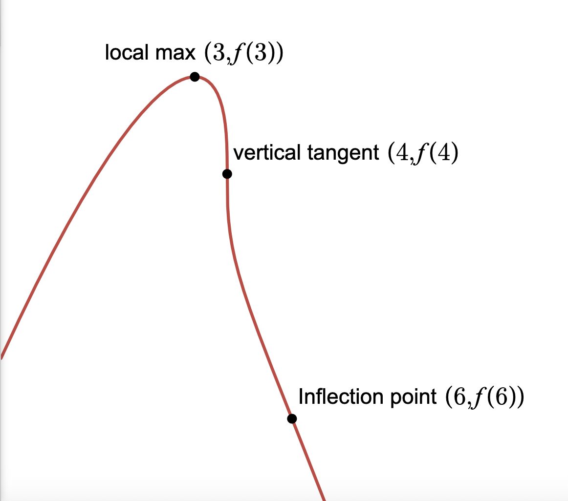
The complete graph of is shown below. Use the graph to answer the following questions.
NOTE: Assume is a local maximum and that is an inflection point.
Figure 6.75
Determine the -values where:
:
:
List the open intervals over which:
:
:
:
:
:
:
Below is the graph of for a continuous function .
Using Example 6.3.5 as a guide, sketch a probable graph of .
Figure 6.76
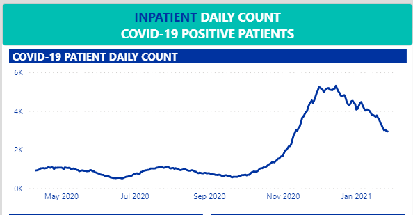
The graph below was taken from https://ohiohospitals.org/covid19data on January 28th, 2021:
Figure 6.77
With help from your classmate, highlight and label one segment on the graph which (roughly) represents the following scenarios.
For brevity, we'll use `patients' to mean `inpatient COVID positive patients' and `the rate of change' to mean `the rate of change of inpatient COVID positive patients with respect to time.'
The number of patients is decreasingand the rate of change is decreasing. (Label this `a.')
The number of patients is decreasingand the rate of change is increasing. (Label this `b.')
The number of patients is increasingand the rate of change is increasing. (Label this `c.')
The number of patients is increasingand the rate of change is decreasing. (Label this `d.')
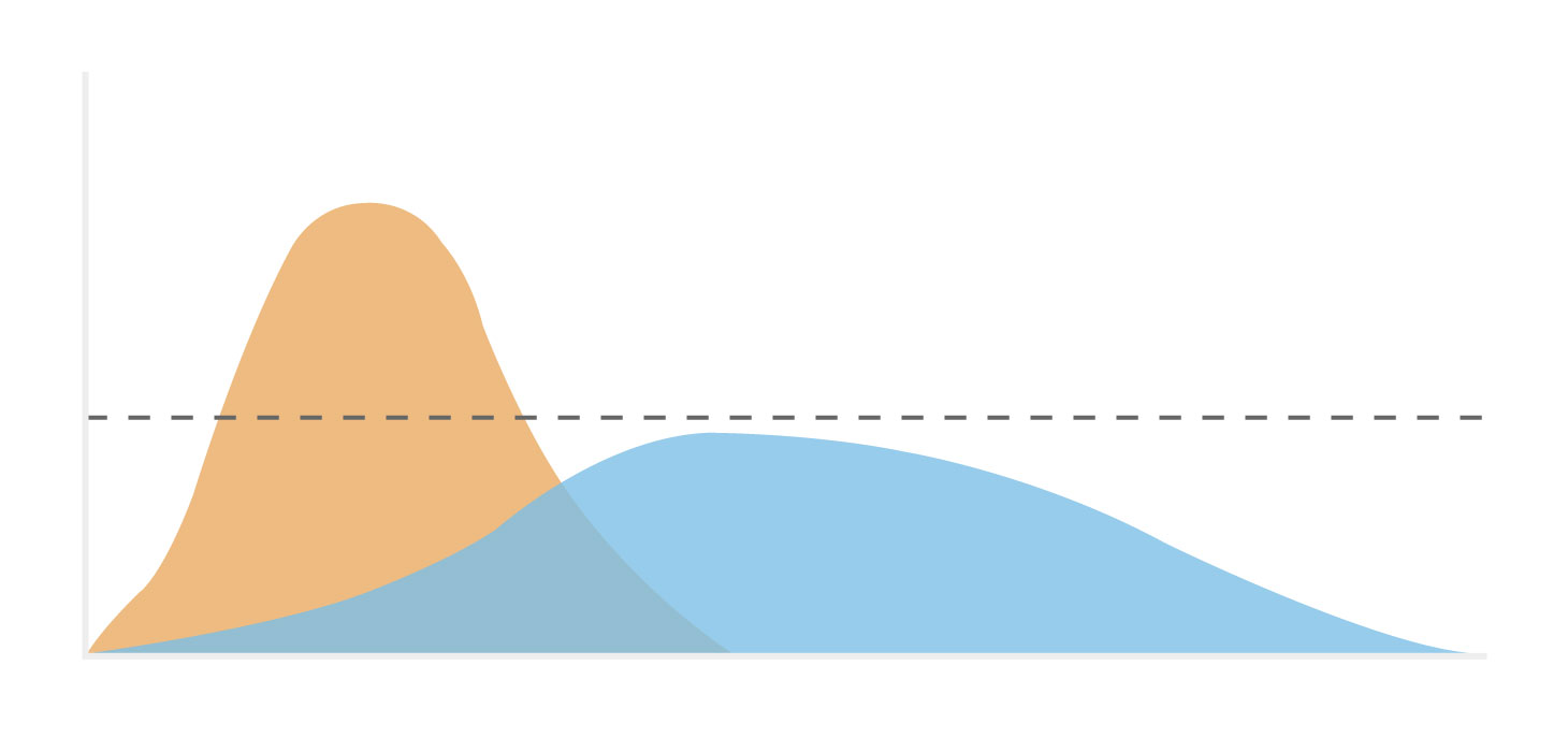
Discuss with your classmates what the phrase `flatten the curve' could mean in terms of first and second derivatives. (See below for an illustration.)
Figure 6.78
Answers
increasing: , ; decreasing: ; local max: ; local min: .
increasing: ; decreasing: , ; local max: ; local min: .
The graph of is a line so we know on one side of , and on the other side, .
Hence, the graph of the original function changes concavity at .
To solve , we set the numerator, . We get so .
Divide both numerator and denominator of by :
and substitute .
If , then:
.
When , we have that and . By the Second Derivative Test for Local Extrema, Theorem 6.7, the average cost has a minimum when
:
: (., too.)
:
: none
:
:
:
: .
Answers vary. below is a sketch of the key features that should be included:
Figure 6.79
Adapted from Precalculus with Integrated Calculus, edition 4i, by Carl Stitz and Jeff Zeager (stitz-zeager.com), licensed under CC BY-NC-SA 3.0. Changes were made: reformatted as an accessible XYZ web edition. License: CC-BY-NC-SA-3.0.
These eBooks are a prerelease and are not yet certified conformant with WCAG 2.1 AA or any other accessibility standard. Every page is built against an automated accessibility gate, and our target for the published editions is WCAG 2.2 Level AA. If something is unusable, please tell us.