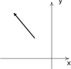
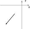
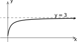
In this chapter, we take some more steps towards1 Calculus. We first revisit the concept of limit. We've primarily used limits as a way to analyze and codify function behavior in places where we simplify could not evaluate the function.2 We first focus on how the concept is expressed graphically.
Limits from Graphs
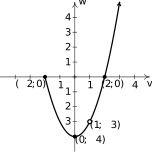
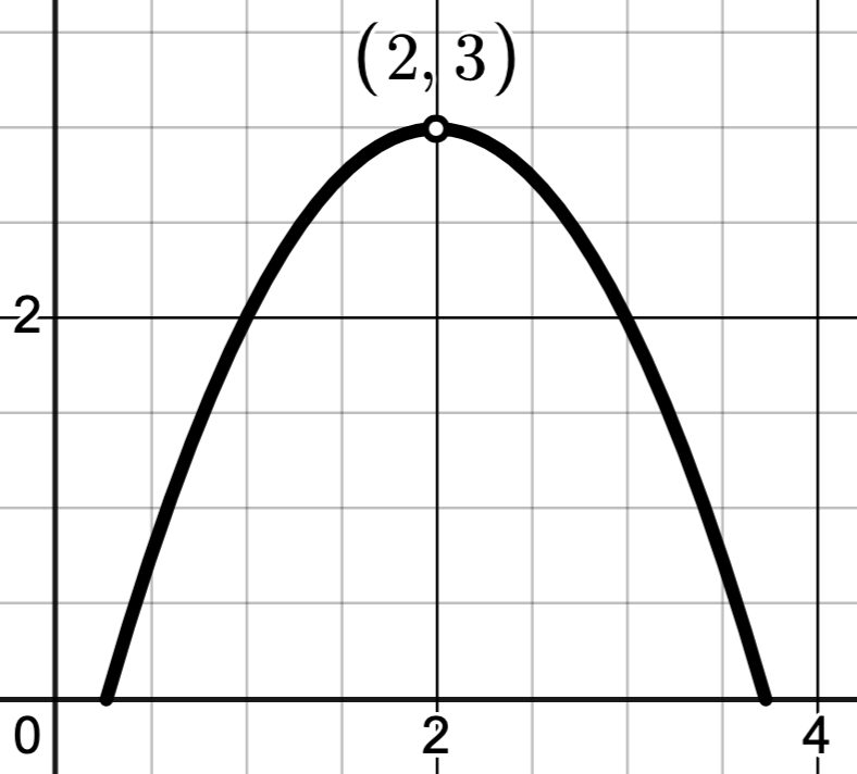
Even though we didn't introduce the limit concept or notation until Chapter 2, we first encounter the underlying concept much earlier. Recall in Example 1.1.4 we were given the graph of a function :
Figure 6.1
The hole in the graph tells us that even though is undefined, we'd expect
to be based on what's happening with the graph near the point . Using limit notation, we'd write . We take a moment below to better define what we mean when use the limit notation.
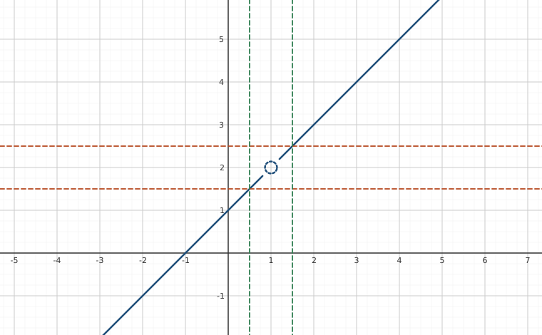
Interactive figureA limit as a window: every ε band has a δ corridor that fits inside itDrag the Tolerance ε, with δ = ε slider from 0.05 to 1.5.
XYZ Graph · viewer build 5edf91b
The function is (x² − 1)/(x − 1), the line y = x + 1 with a hole at x = 1 marked by the hollow circle, so the limit as x approaches 1 is 2 even though f(1) is undefined. The two dashed rust lines are the band 2 − ε < y < 2 + ε around the limit value, and the two dashed green lines are the corridor 1 − δ < x < 1 + δ around the point. Because the slope is 1, choosing δ = ε works: every x in the corridor except 1 itself sends f(x) into the band. Slide ε toward zero and both the band and the corridor tighten around the hole together, which is the whole content of the formal definition.
Some remarks about Definition 6.1 are in order. Note that the business about being defined on `an open interval containing ' is there to guarantee that we have the appropriate `room' for inputs to approach from either direction.4 (For now, we'll just assume we all understand what the word `approach' means in this context and let a Calculus class explain how this is more precisely codified mathematically.)
The phrase `except possibly at ' which immediately follows means the limit doesn't concern itself with what is actually happening at . The function may or may not be defined at . Indeed, if , could be , could be a number different than or could not be defined.
This drives home the principle difference between the precalculus notion of `' and the Calculus notion of `': `' is what we expect
to be - which may or may not agree with what , if is even defined.
For example, using the graph from Example 1.1.4, we write since as , we see . In this particular case, so we get from at what we expect to get.5
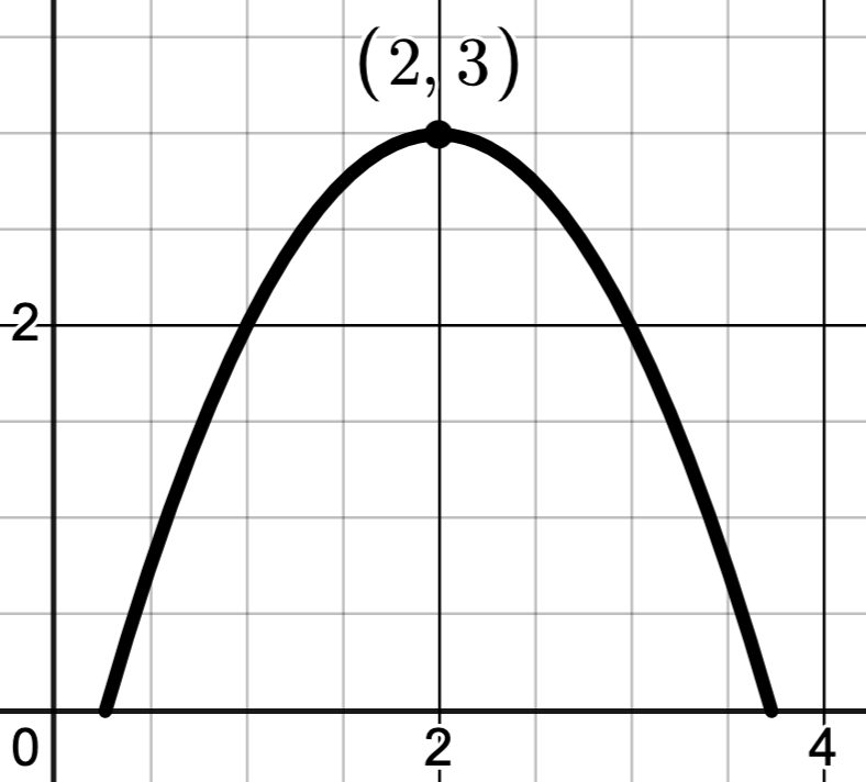
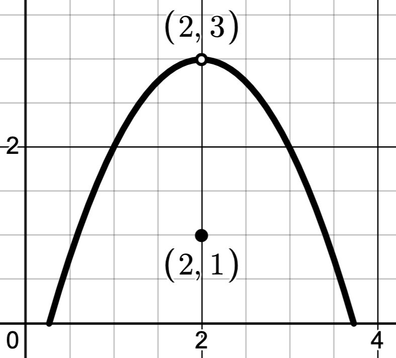
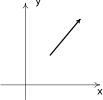
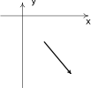
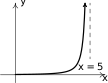
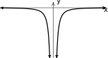
For another example, consider the graphs of the functions , , and below near . Through a precalculus lens, each of these functions is different at : , , and is undefined. Through a Calculus lens, however, all three of these functions are behaving identically as approaches : , , and .
Figure 6.2Figure 6.3Figure 6.4
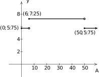
Next let's head to Section 1.2 and revisit Example 1.2.1 in a piecewise-defined function is used to model matinee admission prices at a local theater:
Figure 6.5
What can be said about ? Remember, is what we would expect
to be by analyzing as , ignoring what is happening at . If , is always , so, based on this information, we'd expect
to be . If , then is always , so we'd expect to be . Since Definition 6.1 requires the values to approach a single value as , we'd say in this case that does not exist.
Even though does not exist, we've used so-called `one-sided' limit notation in Chapters 3 and 4 which we can apply here. Specifically, we write and to more precisely record the behavior of as we approach from either direction.6
In order for the (two-sided) limit to exist, both one-sided limits need to exist, be equal, and vice-versa. This is recorded in the following theorem.
It's time for an example.
Another use of limits we've seen is to codify unbounded behavior. Since and aren't real numbers, we used limit notation to help us describe end behavior (as or ) and unbounded function behavior ( or .) Let's take a moment to think about what it means to write . How does one `approach' infinity anyhow?
Let's consider . What me mean here is that as grows larger and larger (without bound), follows suit. To prove something like this, we'd need to show that for any `arbitrarily large' real number, , we can find some threshold so that if the inputs, , the outputs, . For example, if we set , then to guarantee , we can solve and get . So provided , . In this case, and . In general, if , , which justifies us writing .
We can adjust the inequality signs in the sort of argument8 above to direct or to either or . Doing so gives us the (formal) definitions of below.
We'll explore Definition 6.3 more in the Exercises. In the meantime, the reader is encouraged to take some time and think about the inequalities in Definition 6.3 and how they force the corresponding graphical behavior showcased below:
Figure 6.7Figure 6.8Figure 6.9Figure 6.10
Combining the ideas of what it means for or to approach (finite) real numbers along with our (more precise notion) of what it means for or to approach or , we can mix and match to produce expressions and graphs containing vertical and horizontal asymptotes such as the ones depicted below:
Figure 6.11Figure 6.12Figure 6.13
We would be remiss in our duties as (pre)Calculus instructors if we failed to point out that even though we've used notation `' in expressions like above, since is not a real number, technically, does not exist. The `' here just codifies better the manner in which the limit fails to exist.
Our last example of this section turns the tables and has you construct the graph of function given information provided by limits.
Limit Properties and an Introduction to Continuity
Let . Consider . Since the function values are unchanging, there is no other value other than `' to expect from so it stands to reason that . Indeed, for any real number , . In general, if is a constant function, . The formal proof of this fact requires a formal definition of limit,but for now, we'll just take it as true.
Next, let's consider . Consider . What do we expect the value of `' to be as ? Well, `'. Indeed, it can be proved that for all real numbers, .
What about ? Since and , it stands to reason that
which is indeed the case. It turns out that in most cases, limits do respect arithmetic:
For those interested, the Scalar Multiple Rule and Power Rule are grouped with the Product Rule since they both follow directly from the Product Rule. For instance, using the Product Rule,
For powers, note that so that
Once this is established, we can use the fact that and the product rule again to get
Continuing in this manner gives us the Power Rule.10
A note regarding the Rules for Radicals: since is not real if , we have to be careful about limits involving even-indexed radicals (or exponents which indicate even-indexed radicals.) For example, consider . Since this is a `two-sided' limit, we must consider both and .
As , the radicand, so is defined as a real number. More specifically, as , the quantity so . On the other hand, if , the quantity , and is no longer a real number. Therefore, , and, hence, does not exist.
Note the Real Number Powers rule can be thought as a generalization of the Power Rule, Quotient Rule, and Rules for Radicals for the case . Recall that positive rational number exponents can be defined in terms of natural number powers and radicals as: . Negative exponents can be defined in terms of quotients: . For the Real Number Exponents rule, we are generalizing the exponents to any real number but keeping the stipulation that to make sure the resulting answer is defined.11
We put the limit properties to good use in the following example.
It is worth noting that we could have arrived at the same (correct) answer to Example 6.1.3 by evaluating : . That's really the power of Theorem 6.2. Under `nice' circumstances,12 Theorem 6.2 allows us to compute limits using direct substitution. Functions with this property have a familiar name.
This is not the first time we've mentioned this property of functions. Indeed, we've discussed continuity albeit in graphical terms throughout Chapters 1 through 4. In those chapters, we described continuous functions as those whose graphs are connected meaning they have `no holes or breaks' in them. It is a great exercise to compare the description given in Definition 6.4 to the graphical description to see how those two ideas mesh.
In a standard Calculus course, you'll explore properties of continuous functions more extensively. For our purposes here, polynomial, and, more generally, rational functions are continuous on their domains, as well as the functions we encountered in Chapter 4. Indeed, so long as we avoid the usual domain pitfalls, combining continuous functions via the standard four operation function arithmetic or using function composition results in a continuous function. This means in order to evaluate limits of these functions, we may use Definition 6.4 and simply evaluate the function at the corresponding value.
It is worth noting that despite each `piece' of the piecewise-defined function in Example 6.1.4 being continuous, the pieces don't match up at causing what is called a discontinuity. A discontinuity is a place where a function is not continuous. The particular variety of discontinuity appearing here is usually called a `jump' discontinuity - a type of discontinuity belonging to a larger class of `non-removable' or `essential' discontinuities. We'll point out other types of discontinuities as we encounter them.14
We close this section with an example that ties (most of) the fundamental concepts of limits and their calculations together.
The above reasoning is sound and is true in general. We'll be getting a lot of use out of the following:
Exercises
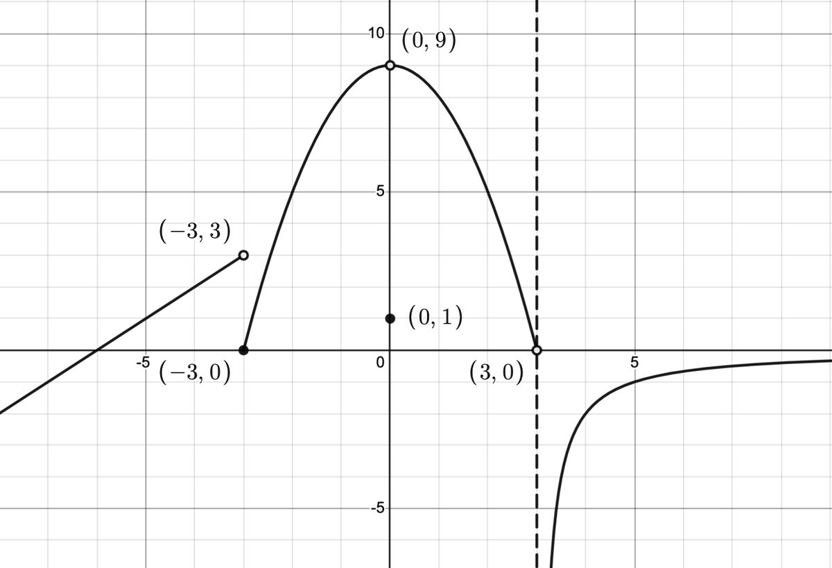
Consider the complete graph of the function below. Use the graph to find the indicated values.
If a limit fails to exist, state that is the case or use the symbols `' or `' appropriately.
NOTE: The graph has a vertical asymptote .
Figure 6.19
Answer
d.n.e.
Explain why if exist, then so do and .
Find an instance19 where and both exist but does not.
Answer
If exists, say then the values approach as from both directions. Hence both one-sided limits exist. In particular, and .
In Example 6.1.1, and both exist but does not because the two one-sided limits are not equal.
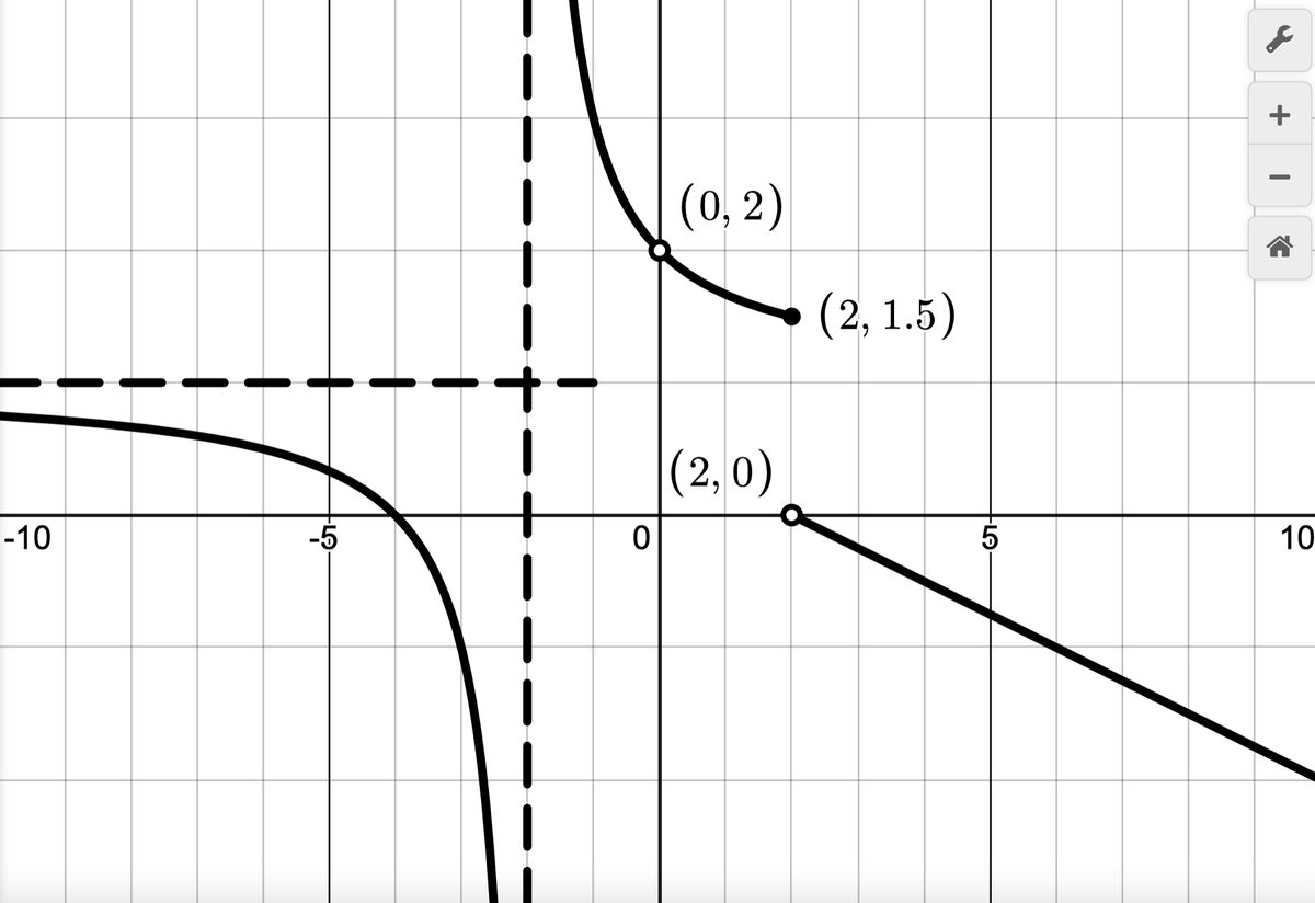
Consider the complete graph of the function below. Use the graph to find the indicated values.
If a limit fails to exist, state that is the case or use the symbols `' or `' appropriately.
NOTE: The graph has a vertical asymptote and a horizontal asymptote .
Figure 6.20
Answer
For Exercises -, find the limit analytically using Exercise 6.1.5 as a guide. If a limit fails to exist, state that is the case or use the symbols `' or `' appropriately.
Answer
Answer
Answer
does not exist
Answer
Answer
Answer
For Exercises -, use the piecewise definition of absolute value, Definition 1.9 to help you find the limit analytically. If a limit fails to exist, state that is the case or use the symbols `' or `' appropriately.
Answer
Answer
For Exercises -, simplify the complex fraction in order to help you find the limit analytically.20 If a limit fails to exist, state that is the case or use the symbols `' or `' appropriately.
Answer
Answer
Answer
For Exercises -, rationalize the numerator of the fraction in order to help you find the limit analytically.21 If a limit fails to exist, state that is the case or use the symbols `' or `' appropriately.
Answer
Answer
Answer
In Exercises -, find the limit analytically. Use the symbols `' and `' as appropriate.
Answer
Answer
Answer
Answer
Answer
.Answer
Let where `' is the greatest integer (or floor) function.22
Fill in the blanks below to help you analyze .
If , then . So we can rewrite .
Using part (a), we can find .
If , then , hence does not exist as .
Putting parts (b) and (c) together, we have that
Graph on desmos near to confirm your answers.
Answer
If , then . So we can rewrite .
Using part (a), we can find .
If , then , hence does not exist as .
Putting parts (b) and (c) together, we have that does not exist.
Sketch the graph of a function which satisfies all of the following criteria:
Answer
Answers vary.
Sketch the graph of a function which satisfies all of the following criteria:
Answer
Answers vary.
A function is said to be continuous from the left at if . Likewise, a function is said to be continuous from the right at if .
Explain why is not continuous at . Is continuous from the left at ? From the right? Explain.
Explain why the floor function23
is not continuous at . Is continuous from the left at ? From the right? Explain.
If a function is continuous at , explain why is continuous from both the left and the right at . Is the converse true? That is, if is continuous from both the left and the right at , is continuous at ?
Compare and contrast your answers in this exercise to those in Exercise.
Answer
The function is not continuous at since is undefined if , so does not exist. However, is continuous from the left at since
.
The function is not continuous at since but . However, is continuous from the right at since .
If is continuous at , then . This means and , so is continuous from both directions at . The converse is also true since ff and , then .
The difference between the scenario here and that in Exercise is that here, we know what each of the one-sided limits are: . They can't be different numbers like they could be in Example 6.1.1
Consider the table of values below:
It turns out that . How is this possible assuming the data in the table is correct?
Answer
We are told nothing of the function on the interval so the function has plenty of opportunities to approach .
In this exercise, we use Definition 6.3 to prove and :
Solve the following inequalities:
Show that for , if , then . Write a sentence (or two!) which uses your work and Definition 6.3 to prove .
Repeat a similar argument to prove
Answer
for .
for .
for .
for .
If , then . Per Definition 6.3, given , choose . If , then . Hence, .
Given , choose . If , then . Hence, .
Adapted from Precalculus with Integrated Calculus, edition 4i, by Carl Stitz and Jeff Zeager (stitz-zeager.com), licensed under CC BY-NC-SA 3.0. Changes were made: reformatted as an accessible XYZ web edition. License: CC-BY-NC-SA-3.0.
These eBooks are a prerelease and are not yet certified conformant with WCAG 2.1 AA or any other accessibility standard. Every page is built against an automated accessibility gate, and our target for the published editions is WCAG 2.2 Level AA. If something is unusable, please tell us.