We begin this section by revisiting (again!) the notion of average velocity - a concept we first encountered in Example 1.2.8 in Section 1.2 and later revisited in Example 3.1.3 in Section 3.1.
In this scenario, the position function1
, gives the height of a model rocket above the Moon's surface, in feet, seconds after liftoff. The average rate of change of over an interval is the average velocity of the rocket over that interval. The average velocity provides two pieces of information: the average speed of the rocket along with the rocket's direction. We formalized the average velocity in Definition 3.5 in Section 3.1:
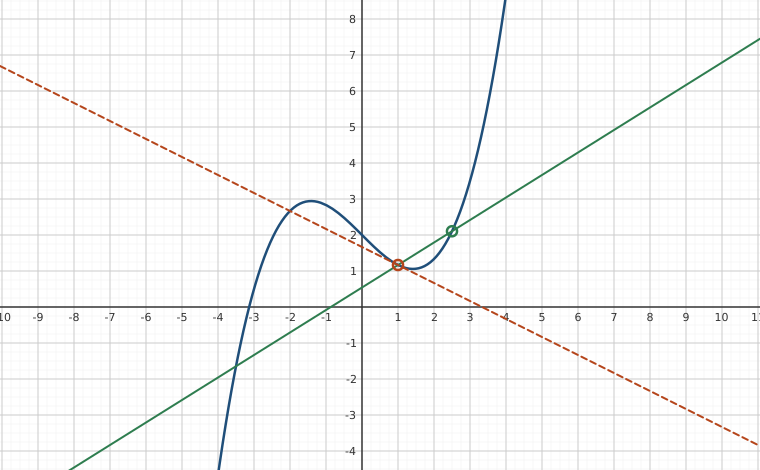
Interactive figureShrink the step h and the secant line settles onto the tangentDrag the Point a and Step h sliders.
XYZ Graph · viewer build 5edf91b
The curve is f(x) = x³/6 − x + 2. The green line passes through the two marked points (a, f(a)) and (a + h, f(a + h)), so its slope is the difference quotient (f(a + h) − f(a))/h, the average rate of change over the step. The dashed line is the tangent at a, whose slope is the derivative f′(a) = a²/2 − 1. Slide h toward zero and the second point slides into the first while the green secant rotates onto the dashed tangent; slide a and both points ride along the curve, the tangent tilting with the curve's local direction.
If we define the change in time, , we get which gives:
The above formula measures the average velocity between time and time as a function of .
We now revisit Example 3.1.3 in Section 3.1 using this new formulation.2
The reader is invited to compare Example 3.1.3 in Section 3.1 with Exercise 6.2.1 above. We obtain the exact same information because we are asking the exact same questions - they are just framed differently. We now take the time to formally define instantaneous velocity:
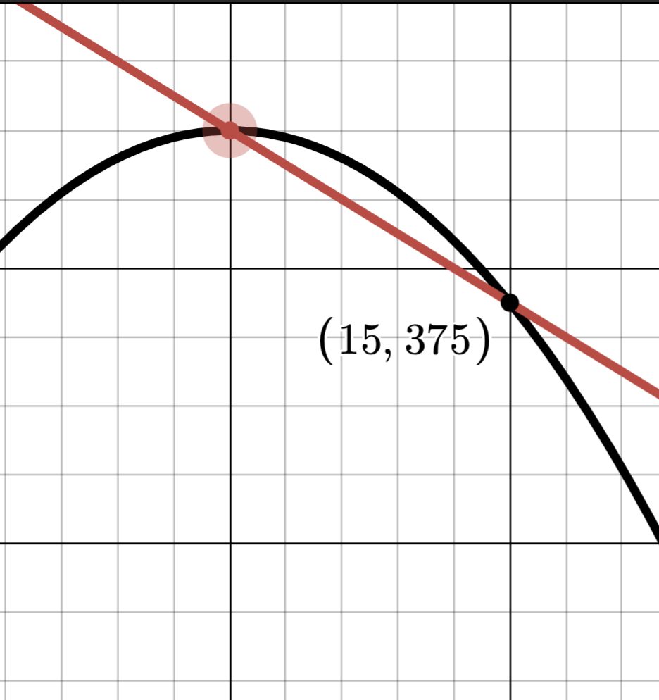
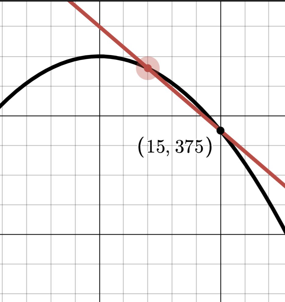
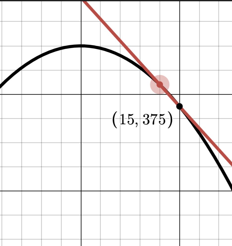
Based on our work in Examples 3.1.3 and 6.2.1, we have . In both of those examples, we've seen what means on the graph of , but there is a more important interpretation when we analyze the graph of . Recall that the average velocity, and, more generally, average rates of change can be visualized as slopes of secant lines.3
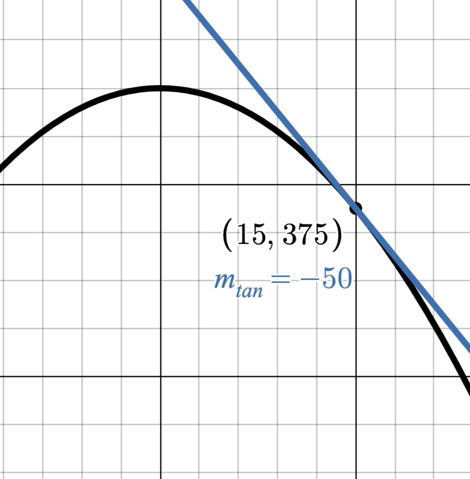
Below is a sequence of secant lines along with the graph of . In each case, the secant line is graphed between and another point on the graph.4 As the points on the parabola approach the secant lines approach what is known as the tangent line.
Figure 6.22Figure 6.23Figure 6.24
To find the equation of the tangent line in this case, which we'll call , we refer to the point-slope form of a line, Equation 1.1:
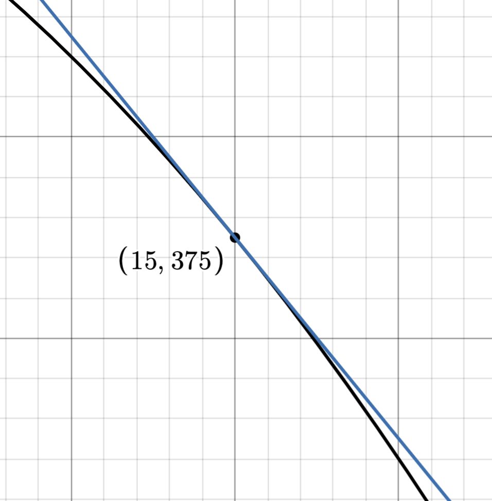
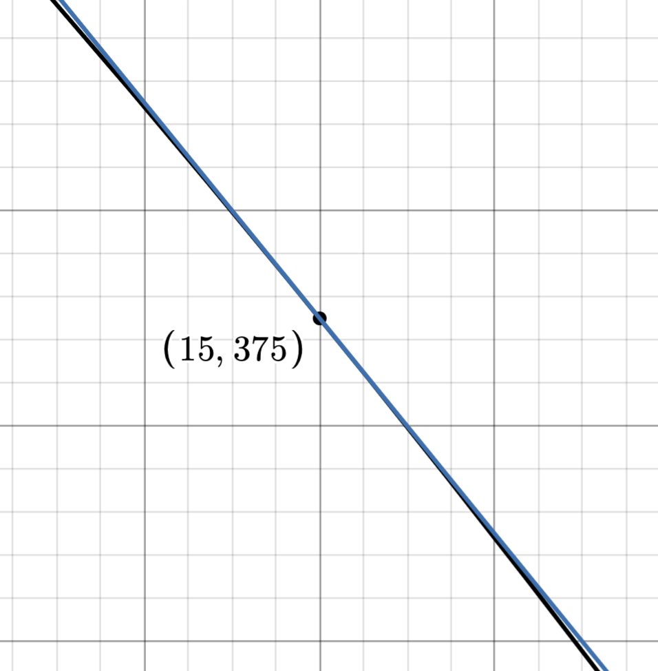
The tangent line can best be thought of as `the best linear approximation' to the graph of at . That is, if we zoom in near , the graph of and this tangent line become indistinguishable. This geometric property of is called local linearity5 and is foundational to the analysis of functions. Below we graph along with and observe the local linearity near .
Figure 6.25Figure 6.26Figure 6.27
The tangent line at .
Zooming in near .
Zooming in closer to .
Our next step is to generalize these notions to all functions.
Difference Quotients and Derivatives
Recall in Section 1.2.4 the concept of the average rate of change of a function over the interval is the slope between the two points and and is given by
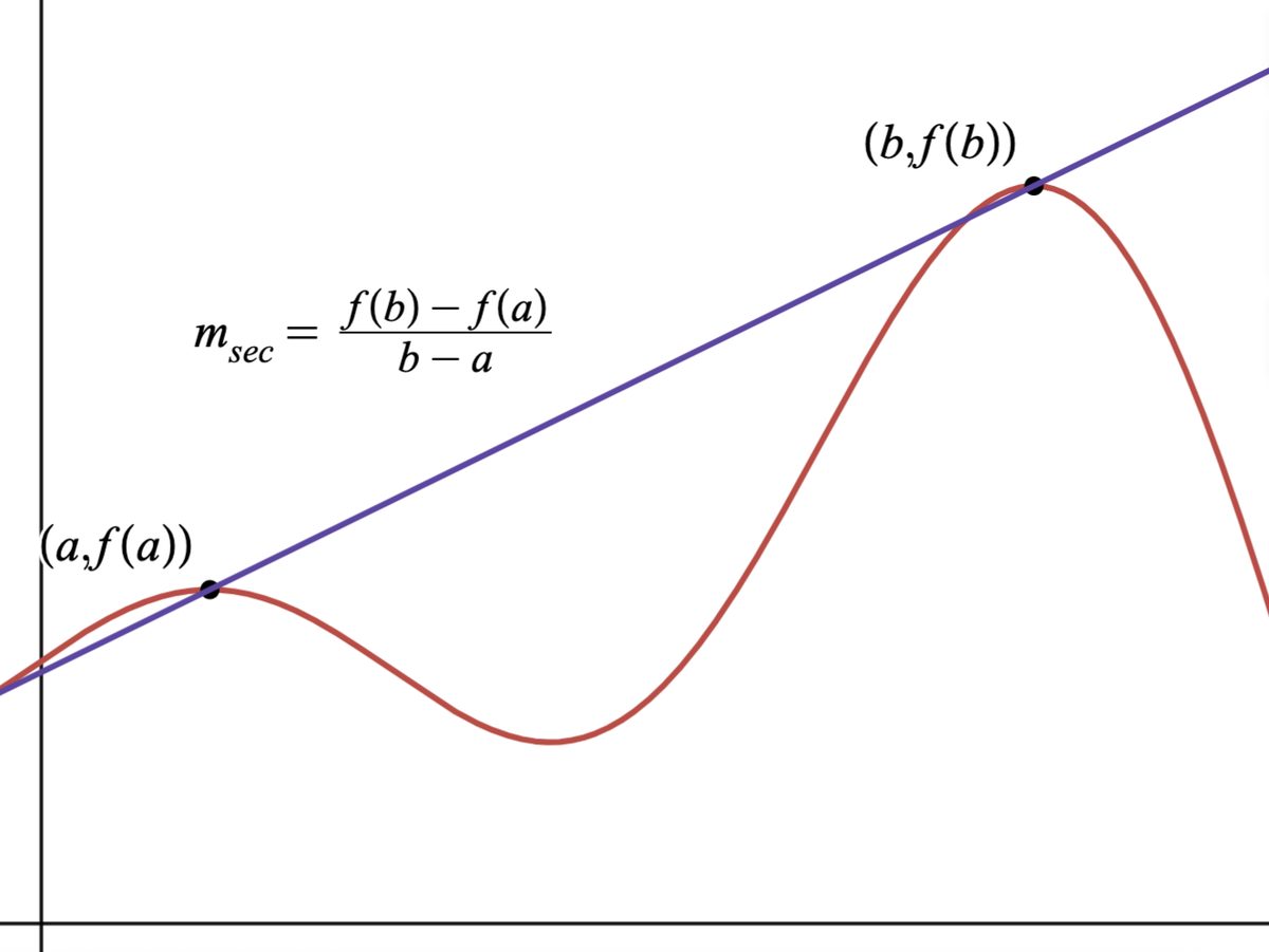
Geometrically, the average rate of change is the slope of the so-called secant line which `cuts' through the graph of at the points and :
Figure 6.28
Consider a function defined over an interval containing and where . The average rate of change of over the interval is thus given by the formula:6
The above is an example of what is traditionally called the difference quotient or Newton quotient of , since it is the quotient of two differences, namely and . Another formula for the difference quotient (as seen in Section 5.2.1) keeps with the notation instead of :
It is important to understand that in this formulation of the difference quotient, the variables `' and `' are distinct - that is they do not combine as like terms.
Note that, regardless of which form the difference quotient takes, when , , or is , the difference quotient returns the indeterminate form `.' As we've seen with rational functions in Section 3.1, when this happens, we can use a limit to help us determine the indeterminate form.
In Section 6.2.1, taking the limit of average velocity as produced instantaneous velocity. More generally, taking the limit of the average rate of change as the denominator approaches produces the instantaneous rate of change of the function at that point. The instantaneous rate of change of a function, called the derivative of the function, is defined below.
Using the language of derivatives, Examples 3.1.3 and 6.2.1 have us computing . Moreover, since the derivative is a rate of change, it's important to note that the associated units of are . This tracks with the units of being , a velocity.
As in Section 6.2.1, represents the slope of the tangent line at the point . We use this to formally define the tangent line below.
We put these definitions to good use in the following example.
What if we wanted to find the equation of the tangent line to the graph of the function in Example 6.2.2 at ? ? ? We'd ostensibly need to run through difference quotients and limit calculations for each and every input value: , , and . Or we could do a single limit with a generic `', simplify the difference quotient and take the limit once, and substitute in particular values of :
It is worth noting that if we set , and consider the graph , we get:
which is why sometimes the derivative is denoted7
.
The astute reader will note that the graph of in Example 6.2.3 is a parabola and finding where lead us right back to the vertex. Using a derivative to find the vertex may seem a bit excessive given that we've algebraically derived a handy `vertex formula' in Section 1.4. However, as the functions we aim to analyze become more and more sophisticated, the tools we use to analyze them must also become more sophisticated. The derivative is one such tool that has a near universal application.8
Exercises
In Exercises -, find the limit of the following difference quotients.
In Exercises -, find:
The equation of the tangent line at . Check your answer graphically.
The equation of the tangent line at . Check your answer graphically.
Find for where
Find for where .
Solve for . Does this look familiar? Explain.
In Exercises -, find the limit of the following difference quotients:
In Exercises -, find the limit of the following:
The equation of the tangent line at .
The equation of the tangent line at .
In Exercises -, find the limit of the following difference quotients:
In Exercises -, find the following:
The equation of the tangent line at .
The equation of the tangent line at .
For :
Explain why does not exist.
Find the derivative from the right at :
Find and interpret.
Find . Assume .
Find for , .
What restrictions do you place on so your formula is valid?
Let .
Explain why is continuous at .
Show does not exist by showing but .
Graph near . Interpret your answer to number graphically.
Find and simplify assuming .
HINT: Consider the two cases and …
Let .
Explain why is continuous at .
Show does not exist by showing .
Graph near . Interpret your answer to number graphically.
Find and simplify assuming .
HINT:
Let .
Explain why is continuous at .
Show does not exist by showing and
Graph near . Interpret your answer to number graphically.
Find and simplify assuming .
HINT:
and .
Recall from Exercise in Section 1.4 that Carl's friend Jason participates in the Highland Games. In one event, the hammer throw, the height in feet of the hammer above the ground seconds after Jason lets it go is modeled by the function .
Find and simplify a formula for the velocity of the hammer, .
Find and interpret .
Solve and interpret.
Find the velocity of the hammer when it hits the ground, rounded to three decimal places.
In Exercise in Section 1.4, the average fuel economy in miles per gallon (mpg) for passenger cars in the US years after 1980 is modeled by , .
Find and simplify a formula for .
Find and interpret , and .
Interpret the trend you observe in your answers to part.
Let us return to Example 5.2.4 where denotes the cost, in dollars, of producing PortaBoy game systems.
Find and interpret .
Recall in Exercise in Section 5.2, we found the marginal cost, , which means it will cost an additional to produce the th item. Compare and .
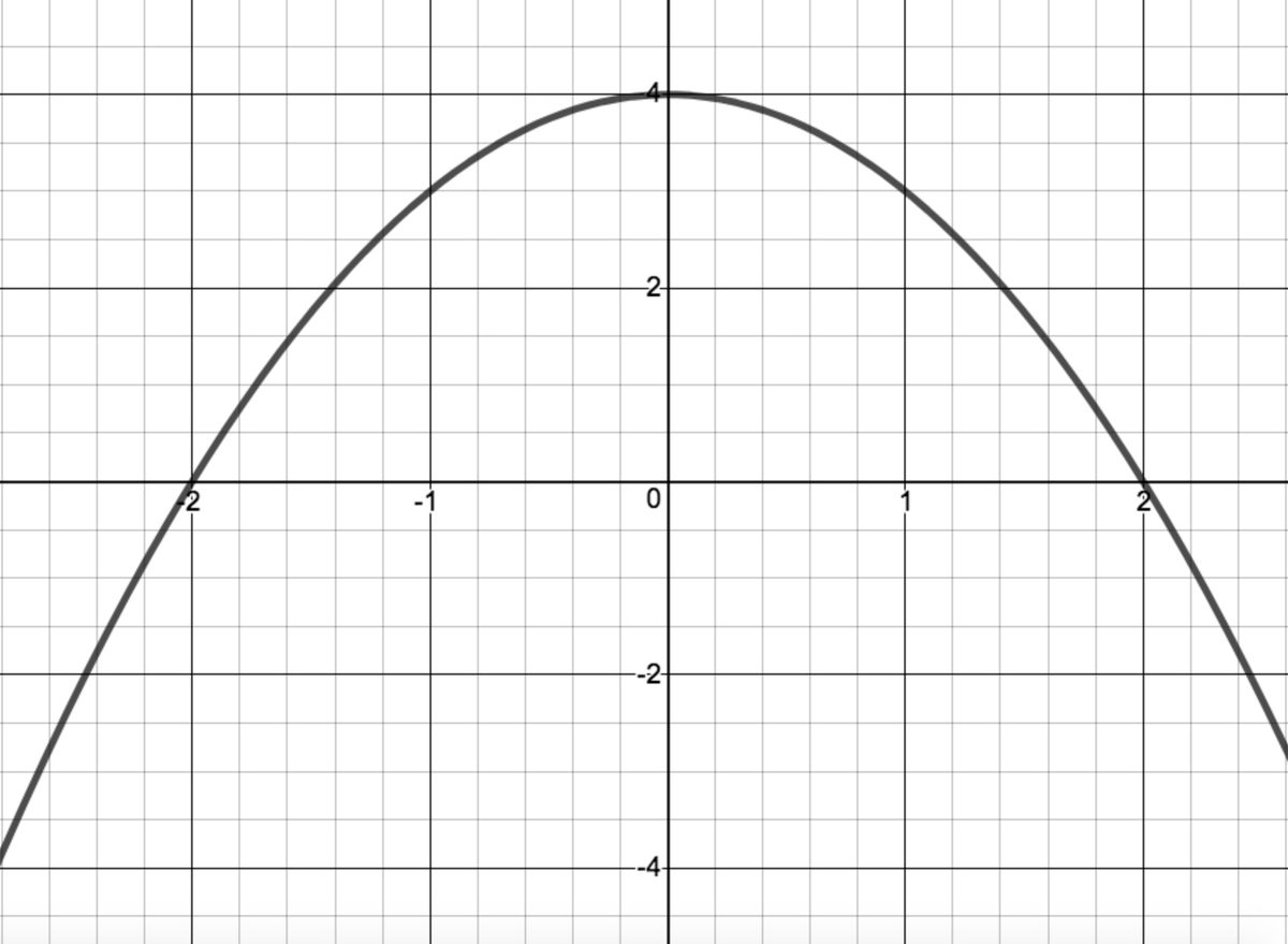
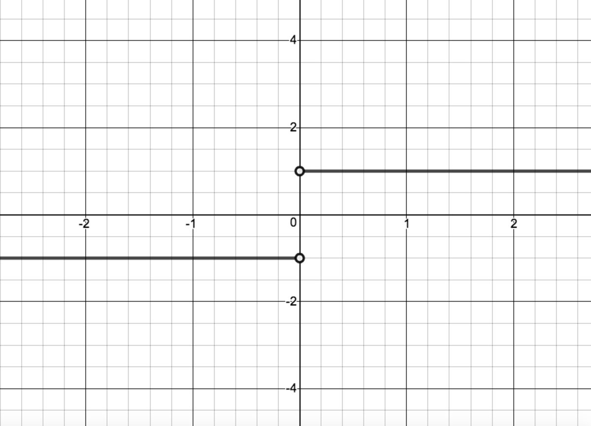
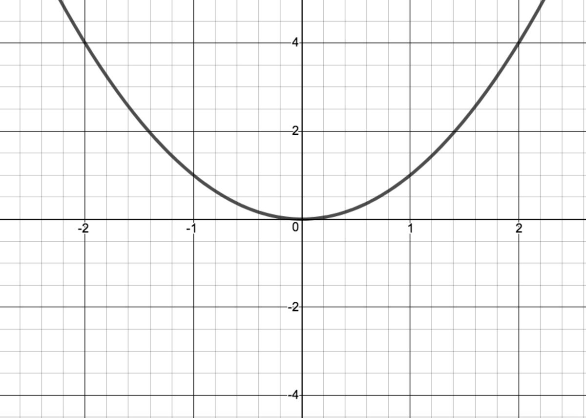
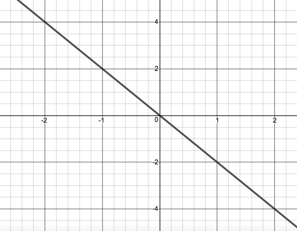
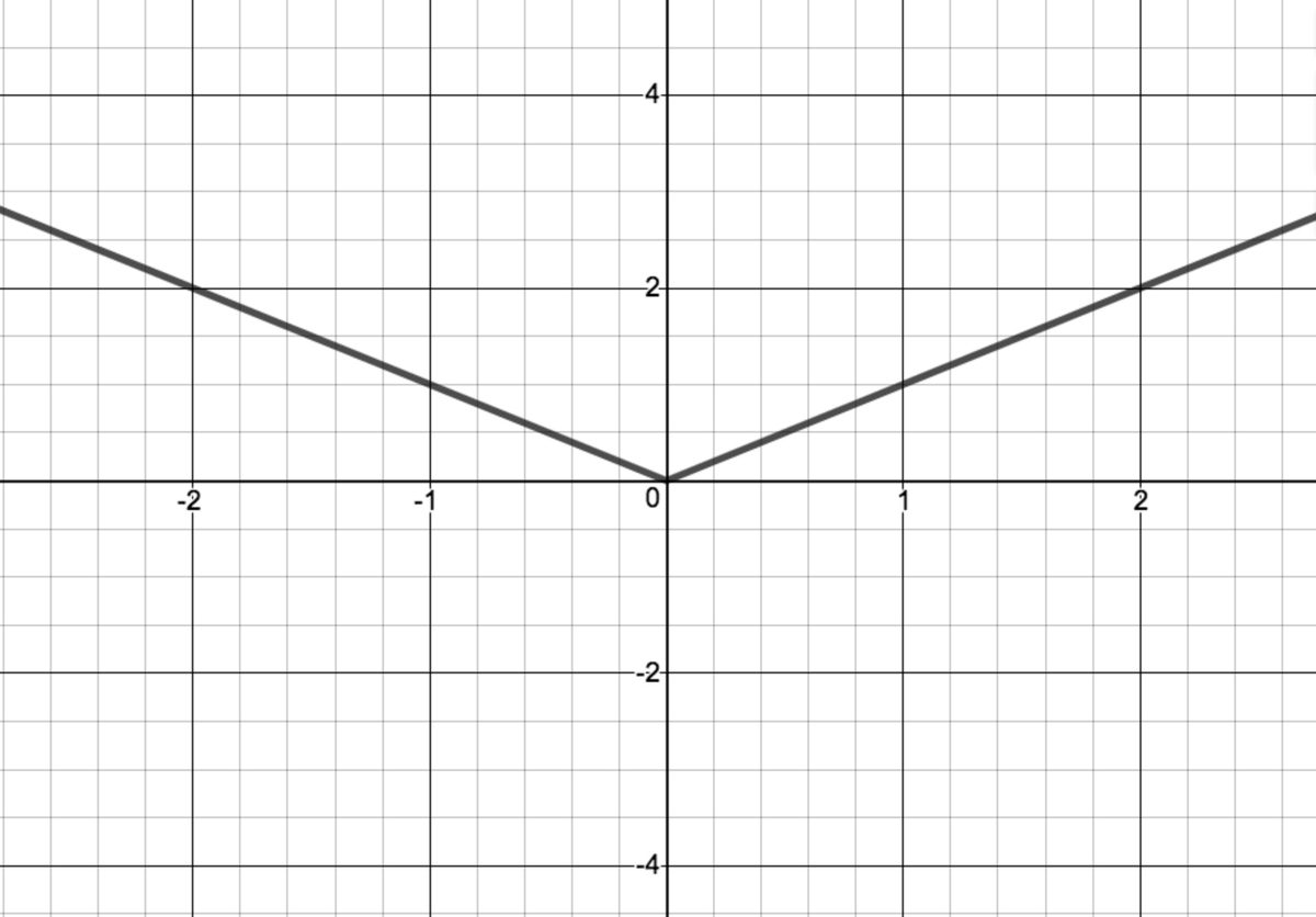
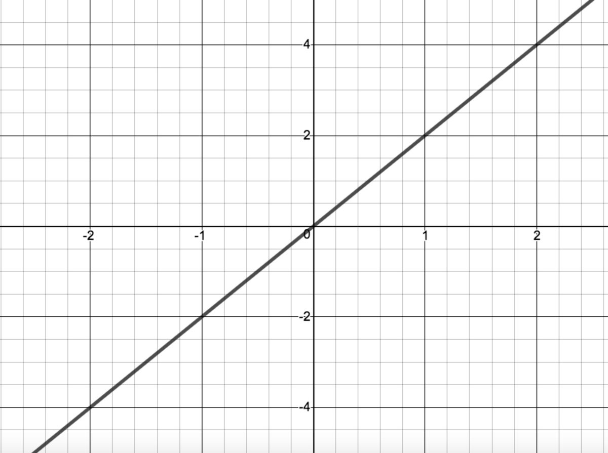
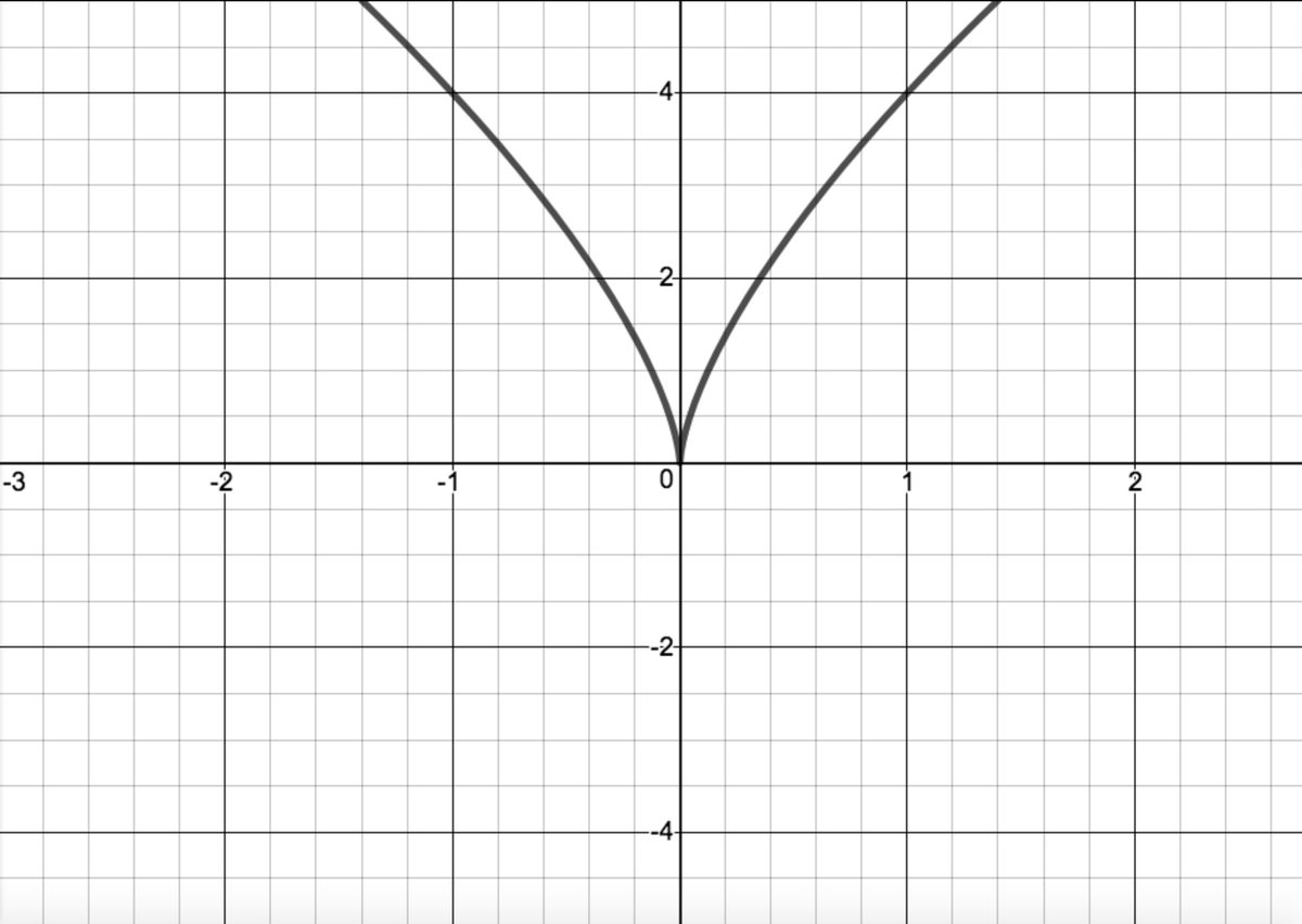
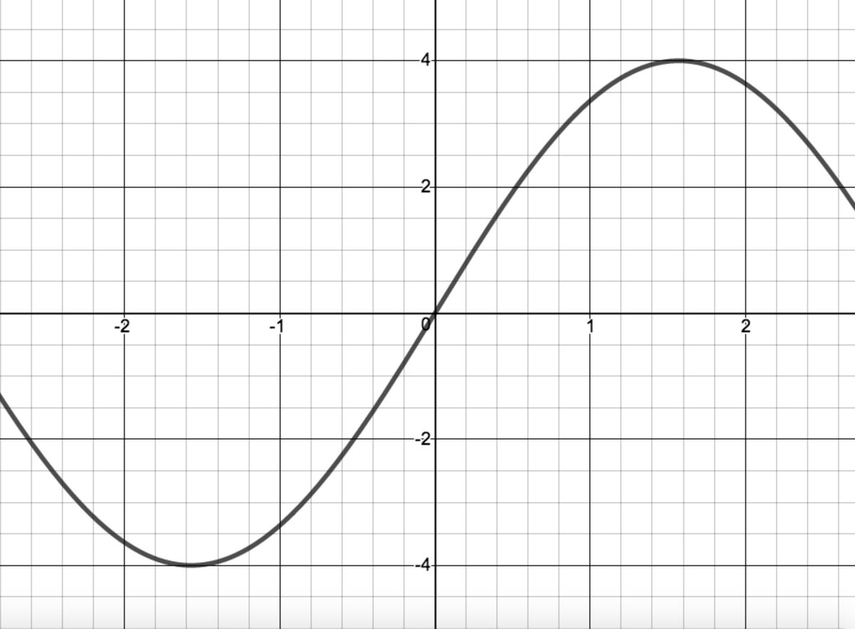
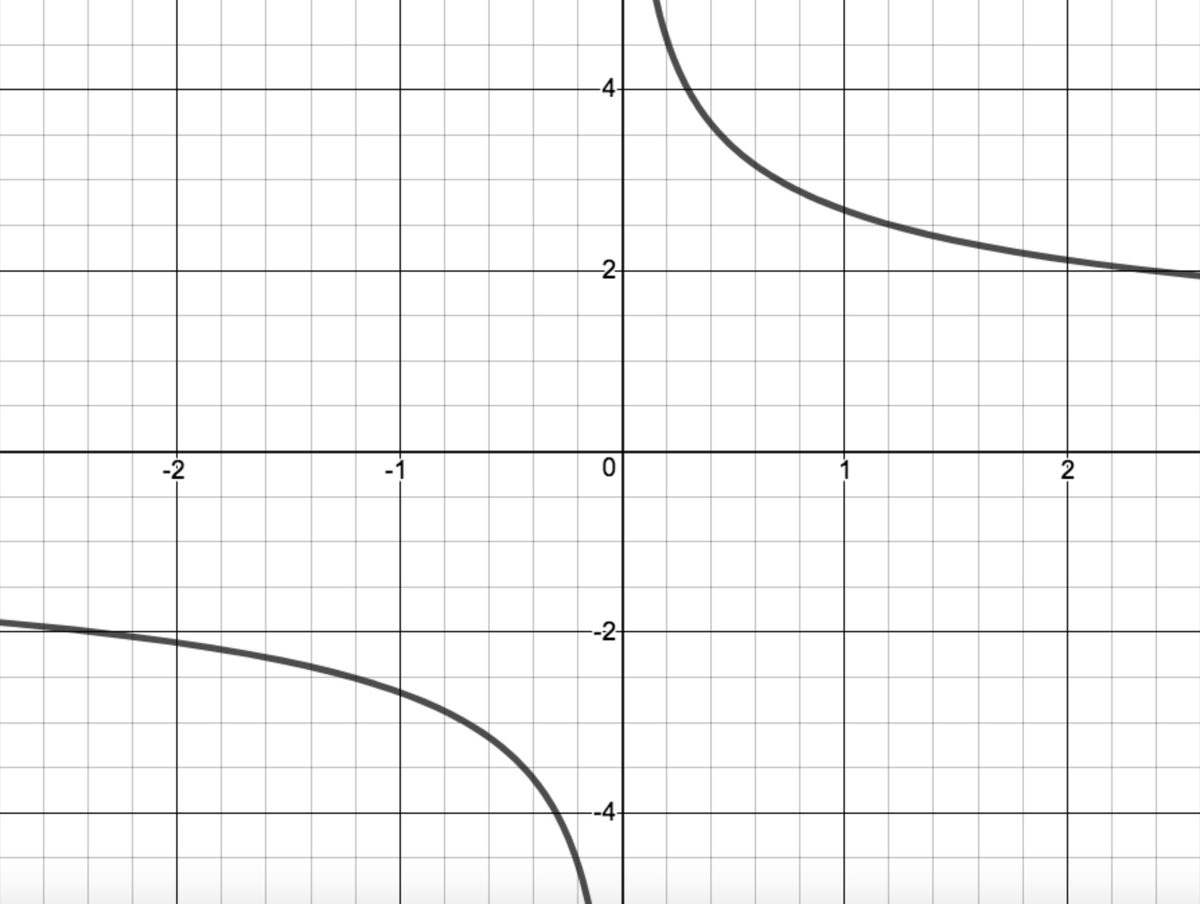
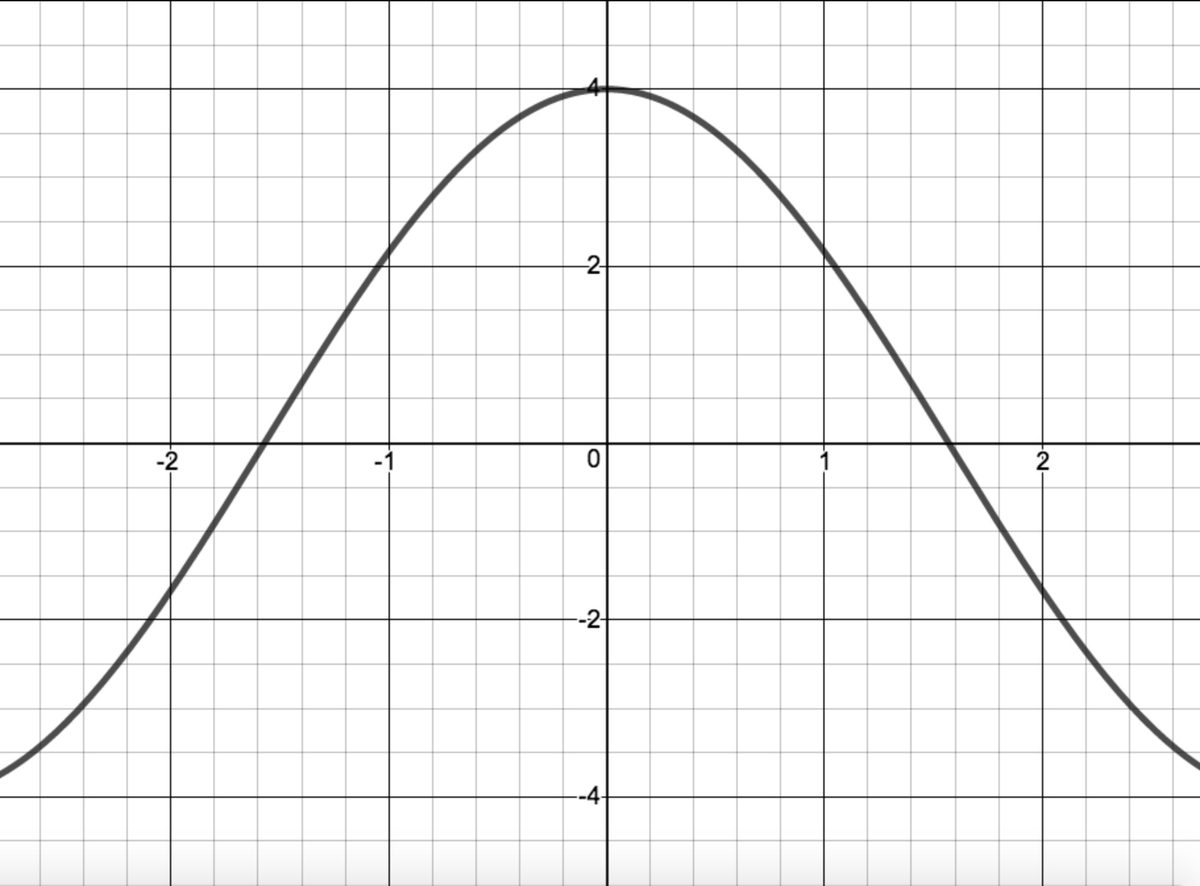
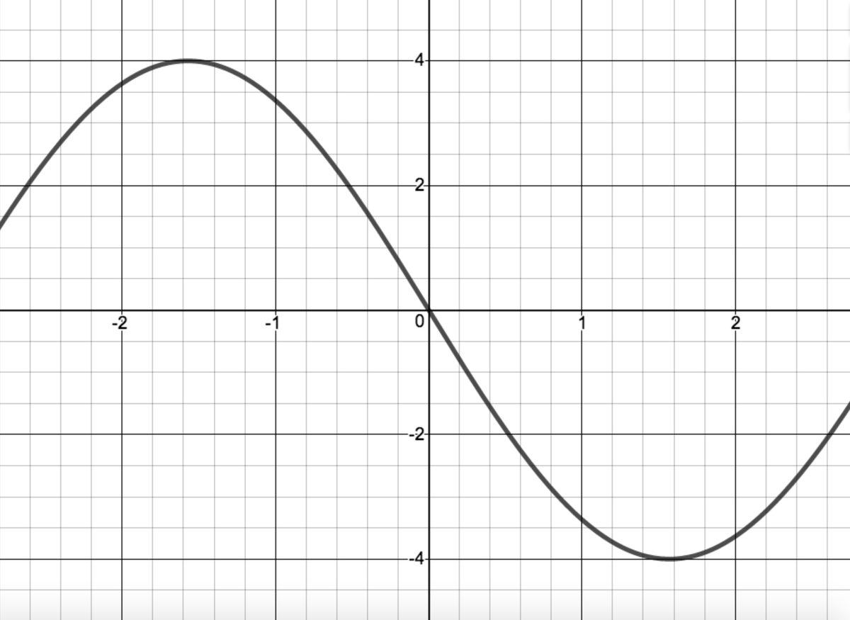
In Exercises -, match the graph of the function with a plausible graph of its derivative.
:
Graph A:
Figure 6.38Figure 6.39
:
Graph B:
Figure 6.40Figure 6.41
:
Graph C:
Figure 6.42Figure 6.43
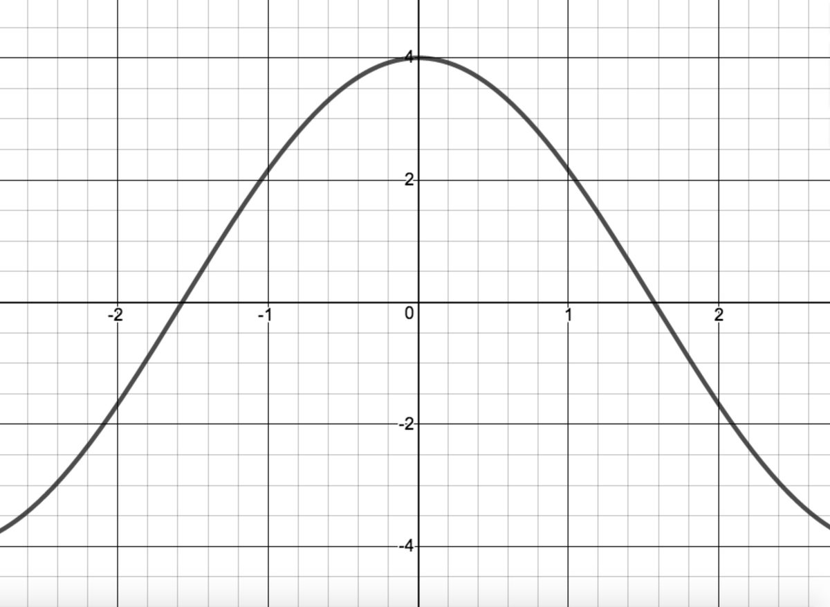
In Exercises -, match the graph of the function with a plausible graph of its derivative.
:
Graph A:
Figure 6.44Figure 6.45
:
Graph B:
Figure 6.46Figure 6.47
:
Graph C:
Figure 6.48Figure 6.49
Answers
,
, ,
,
,
,
,
so .
so .
so .
so .
.
.
Solving for gives which is the formula for the -coordinate of the vertex of the parabola . If we zoom in near the the vertex of a parabola, the graph becomes locally flat so it makes sense the slope of the tangent line, there.
,
,
,
,
so .
so .
so .
so .
so .
so .
so .
so .
,
,
so .
so .
so .
so .
If , then is not a real number. Hence, does not exist.
so .
This line is a tangent line to the graph of at for .
provided .
.
We are told . In order for the square roots to be happy, we assume . Hence, if and if .
is continuous at since .
,
Near , the graph of looks like a `' shape12 consisting of a line of slope to the left of and a line with a slope of to the right of .
if and of .
is continuous at since .
The graph of near is a vertical line.13 Since is increasing through , the `slope' of this vertical line could be seen as .
, .
.
and
The graph near shows a steeply decreasing graph as we approach from the left followed by a steeply increasing graph as we approach from the right.14
, .
.
. This means initially (when Jason lets go of the hammer), the hammer is traveling upwards at feet per second.
when . This means the (vertical) velocity zeros out seconds after Jason lets go of the hammer. In this scenario, this corresponds to when the hammer reaches its peak height
We first find when the hammer hits the ground by solving . The positive answer here is seconds. The velocity of the hammer is: . The hammer hits the ground going (approximately) feet per second.15
.
, so fuel economy was increasing at a rate of mpg per year in 1980.16
, so fuel economy was increasing at a rate of mpg per year in 1985.
, so fuel economy was increasing at a rate of mpg per year in 1990.
Based on the model, we have that during the years 1980 - 1990, fuel economy was increasing, but less so as the decade wore on. Technical and cost limitations could be at work here.
. This means when producing 75 systems, the cost is increasing at a rate of per system.
We see that is numerically close to but the former is a rate of change (measured in dollars per system) where the latter is a change (measured in dollars). Note that if we set in the difference quotient:
we see these two quantities can be used to approximate each other.
is Graph B
is Graph C
is Graph A
is Graph B
is Graph A
is Graph C
Adapted from Precalculus with Integrated Calculus, edition 4i, by Carl Stitz and Jeff Zeager (stitz-zeager.com), licensed under CC BY-NC-SA 3.0. Changes were made: reformatted as an accessible XYZ web edition. License: CC-BY-NC-SA-3.0.
These eBooks are a prerelease and are not yet certified conformant with WCAG 2.1 AA or any other accessibility standard. Every page is built against an automated accessibility gate, and our target for the published editions is WCAG 2.2 Level AA. If something is unusable, please tell us.