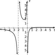
In Section 3.1, we learned about the types of behaviors to expect from graphs of rational functions: vertical asymptotes, holes in graph, horizontal and slant asymptotes. Moreover, Theorems 3.2, 3.3 and 3.4 tell us exactly when and where these behaviors will occur. We used graphing technology extensively in the last section to help us verify results. In this section, we delve more deeply into graphing rational functions with the goal of sketching relatively accurate graphs without the aid of a graphing utility. Your instructor will ultimately communicate the level of detail expected out of you when it comes to producing graphs of rational functions; what we provide here is an attempt to glean as much information about the graph as possible given the analytical tools at our disposal.
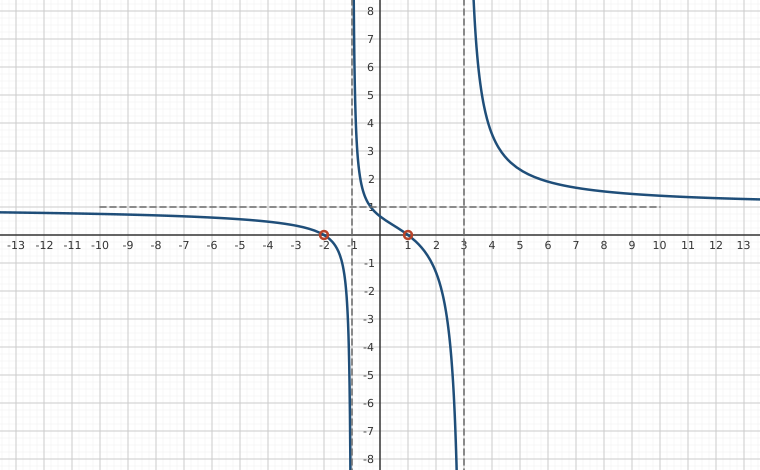
Interactive figureTwo zeros, two poles: the sign diagram drawn as a graphDrag the Movable zero r and Movable asymptote p sliders.
XYZ Graph · viewer build 5edf91b
A rational function with two zeros and two vertical asymptotes, y = (x − r)(x + 2)/((x − p)(x + 1)), where the slider r moves one zero and the slider p moves one asymptote. The dashed vertical lines mark x = p and x = −1, the dashed horizontal line y = 1 is the end behaviour, and the marked points are the x-intercepts. Between any two consecutive marks the graph keeps one sign, which is exactly the sign diagram of the section; drag r across p and watch a zero and a pole trade places, or set r equal to p to cancel a factor and open a hole.
One of the standard tools we will use is the sign diagram which was first introduced in Section 1.4, and then revisited in Section 2.3. In these sections, to construct a sign diagram for a function , we first found the zeros of . The zeros broke the domain of into a series of intervals. We determined the sign of over the entire interval by finding the sign of for just one test value per interval. The theorem that justified this approach was the Intermediate Value Theorem, Theorem 2.14, which says that continuous functions cannot change their sign between two values unless there is a zero between those two values.
This strategy fails in general with rational functions. Indeed, the very first function we studied in Section 3.1, changes sign between and , but there is no zero between these two values - instead, the graph changes sign across a vertical asymptote. We could also well imagine the graph of a rational function having a hole where an -intercept should be.1 With Calculus we can show rational functions are continuous on their domains which means when constructing sign diagrams, we need to choose test values on either side of values excluded from the domain in addition to checking around zeros.2
Steps for Constructing a Sign Diagram for a Rational Function
Suppose is a rational function.
Place any values excluded from the domain of on the number line with an `‽' above them.3
Find the zeros of and place them on the number line with the number above them.
Choose a test value in each of the intervals determined in steps 1 and 2.
Determine and record the sign of for each test value in step 3.
We now present our procedure for graphing rational functions and apply it to a few exhaustive examples. Please note that we decrease the amount of detail given in the explanations as we move through the examples. The reader should be able to fill in any details in those steps which we have abbreviated.
Determine the location of any vertical asymptotes or holes in the graph, if they exist.
Find the axis intercepts, if they exist.
Analyze the end behavior of . Find the horizontal or slant asymptote, if one exists.
Use a sign diagram and plot additional points, as needed, to sketch the graph.5
Something important to note about the above example is that while is the horizontal asymptote, the graph of actually crosses the -axis at . The myth that graphs of rational functions can't cross their horizontal asymptotes is completely false,11 as we shall see again in our next example.
More can be said about the graph of above. It stands to reason that must attain a local minimum at some point past since the graph of crosses through at but approaches from below as . Calculus verifies a local minimum at . We invite the reader to verify this claim using a graphing utility.
Our last graphing example is challenging in that our six step process provides us little information to work with.
Our last example turns the tables and invites us to write formulas for rational functions given their graphs.
Another way to approach Example 3.2.5 is to take a cue from Theorem 3.1. The graph of certainly appears to be the result of moving around the graph of . To that end, suppose . Since the vertical asymptote is and the horizontal asymptote is , we get and . At this point, we have . We can determine by using the -intercept, : gives us so . Hence, . At this point we could check the -intercept is on the graph, check our answer using a graphing utility, or even better, get common denominators and write as a single rational expression to compare with our answer in the above example.
As usual, the authors offer no apologies for what may be construed as `pedantry' in this section. We feel that the detail presented in this section is necessary to obtain a firm grasp of the concepts presented here and it also serves as an introduction to the methods employed in Calculus. In the end, your instructor will decide how much, if any, of the kinds of details presented here are `mission critical' to your understanding of Precalculus. Without further delay, we present you with this section's Exercises.
Exercises
In Exercises -, use the six-step procedure to graph the rational function. Be sure to draw any asymptotes as dashed lines.
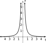
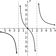
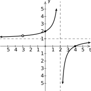
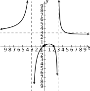
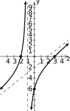
In Exercises -, find a possible formula for the function whose graph is given.
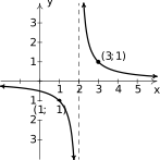
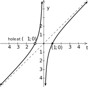
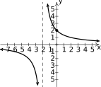
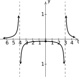
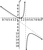
Figure 3.62Vertical asymptote:
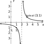
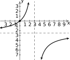
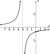
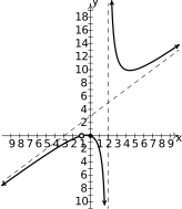
Figure 3.63Vertical asymptote:
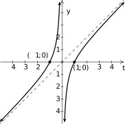
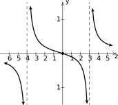
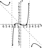
Figure 3.64Slant asymptote:
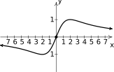
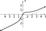
Figure 3.65Slant asymptote:
Let With the help of your classmates:
find the - and - intercepts of the graph of .
find all of the asymptotes of the graph of and any holes in the graph, if they exist.
find the intervals on which the function is increasing, the intervals on which it is decreasing and the local maximums and minimums, if any exist.
sketch the graph of , using more than one picture if necessary to show all of the important features of the graph.
Example 3.2.4 showed us that the six-step procedure cannot tell us everything of importance about the graph of a rational function and that sometimes there are things that are easy to miss. Without Calculus, we may need to use graphing utilities to reveal the hidden behavior of rational functions. Working with your classmates, use a graphing utility to examine the graphs of the rational functions given in Exercises -. Compare and contrast their features. Which features can the six-step process reveal and which features cannot be detected by it?
Answers
Domain: No -intercepts -intercept: Vertical asymptote:
, Horizontal asymptote:
More specifically, as
More specifically, as
Figure 3.66
Domain:
-intercept:
-intercept: Vertical asymptote:
, Horizontal asymptote:
More specifically, as
More specifically, as
Figure 3.67
Domain: No -intercepts No -intercepts Vertical asymptote:
Horizontal asymptote:
More specifically, as
More specifically, as
Figure 3.68
Domain: No -intercepts -intercept: Vertical asymptotes: and
,
, Horizontal asymptote:
More specifically, as
More specifically, as
Figure 3.69
Domain: No -intercepts -intercept:
Hole in the graph at Vertical asymptote:
, Horizontal asymptote:
More specifically, as
More specifically, as
Figure 3.70
Domain:
-intercept:
-intercept: Vertical asymptotes: and
,
, Horizontal asymptote:
More specifically, as
More specifically, as
Figure 3.71
Domain:
-intercept:
-intercept: No vertical asymptotes No holes in the graph Horizontal asymptote:
More specifically, as
More specifically, as
Figure 3.72
Domain:
-intercept:
-intercept: Vertical asymptotes:
,
, No holes in the graph Horizontal asymptote:
More specifically, as
More specifically, as
Figure 3.73
Domain:
-intercept:
-intercept: Vertical asymptote:
, Hole at Horizontal asymptote:
More specifically, as
More specifically, as
Figure 3.74
Domain:
-intercepts: ,
-intercept: Vertical asymptotes:
,
, Horizontal asymptote:
More specifically, as
More specifically, as
Figure 3.75
Domain:
-intercepts: ,
-intercept: Vertical asymptote:
, Slant asymptote:
As , the graph is above
As , the graph is below
Figure 3.76
Domain:
-intercepts:
-intercept: Vertical asymptote:
, Slant asymptote:
As , the graph is above
As , the graph is below
Figure 3.77
Domain:
-intercept:
-intercept: Vertical asymptote:
, Hole at Slant asymptote:
As , the graph is below
As , the graph is above
Figure 3.78
Domain:
-intercepts:
-intercept: Vertical asymptotes:
,
, Slant asymptote:
As , the graph is above
As , the graph is below
Figure 3.79
Domain:
-intercept:
-intercept: Slant asymptote:
As , the graph is below
As , the graph is above
Figure 3.80
Domain: No -intercepts No -intercepts Vertical asymptotes: and
,
, Hole in the graph at Horizontal asymptote:
More specifically, as
More specifically, as
Figure 3.81
Adapted from Precalculus with Integrated Calculus, edition 4i, by Carl Stitz and Jeff Zeager (stitz-zeager.com), licensed under CC BY-NC-SA 3.0. Changes were made: reformatted as an accessible XYZ web edition. License: CC-BY-NC-SA-3.0.
These eBooks are a prerelease and are not yet certified conformant with WCAG 2.1 AA or any other accessibility standard. Every page is built against an automated accessibility gate, and our target for the published editions is WCAG 2.2 Level AA. If something is unusable, please tell us.