If we add, subtract, or multiply polynomial functions, the result is another polynomial function. When we divide polynomial functions, however, we may not get a polynomial function. The result of dividing two polynomials is a rational function, so named because rational functions are ratios of polynomials.
Laurent Monomial Functions
As with polynomial functions, we begin our study of rational functions with what are, in some sense, the building blocks of rational functions, Laurent monomial functions.
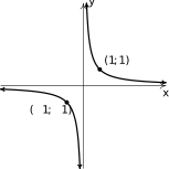
Laurent monomial functions are named in honor of Pierre Alphonse Laurent and generalize the notion of `monomial function' from Chapter 2 to terms with negative exponents. Our study of these functions begins with an analysis of , the reciprocal function. The first item worth noting is that is not defined owing to the presence of in the denominator. That is, the domain of is or, using interval notation, . Of course excluding from the domain of serves only to pique our curiosity about the behavior of when . Thinking from a number sense perspective, the closer the denominator of is to , the larger the value of the fraction (in absolute value.)2 So it stands to reason that as gets closer and closer to , the values for should grow larger and larger (in absolute value.) This is borne out in the table below on the left where it is apparent that for , is becoming unbounded.
As we investigate the end behavior of , we find that as and as , . Again, number sense agrees here with the data, since as the denominator of becomes unbounded, the value of the fraction should diminish.3 That being said, we could ask if the graph ever reaches the -axis. If we attempt to solve . we arrive at the contradiction hence, is not in the range of . Every other real number besides is in the range of , however. To see this, let be a real number. Then is defined and, moreover, . This shows is in the range of . Hence, the range of is or, using interval notation, .
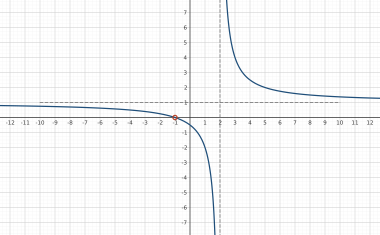
Interactive figureWhere a rational graph breaks: y = (x − a)/(x − b)Drag the Zero a and Vertical asymptote b sliders.
XYZ Graph · viewer build 5edf91b
The simplest rational function with a zero and a vertical asymptote, y = (x − a)/(x − b), with a slider for each. The dashed vertical line x = b is the vertical asymptote, where the denominator vanishes and the two branches run off in opposite directions; the dashed horizontal line y = 1 is the horizontal asymptote, the end behaviour both branches settle toward. The marked point is the x-intercept at x = a. Slide a onto b and the fraction reduces: the asymptote disappears and only a hole is left.
Figure 3.1
Like we did in Section 2.1, we'll borrow some notation from Calculus in order for us to codify the behavior as . First off, note that the behavior of differs depending on which direction we approach . We describe the values but (such as , , etc.) as ` approaching
from the left,' written as . If we think of these numbers as all being -values where , the the `' in the notation `' makes better sense. For these values, the function values . Using the limit notation introduced in Section 2.1, we'd write: .
Similarly, we say `as approaches
from the right,' that is as , , or, more succinctly, . As before, we understand `from the right' means we are using values slightly to the right of on the number line: numbers such as These numbers could described as `,' which justifies the `' in the notation `.'
We can also use this notation to describe the end behavior, but here the numerical roles are reversed. We see as , and as , . When it comes to codifying these results using Calculus, we write and . Note that, unfortunately, we lose the directionality here on the limiting value - that is, we do not write or . Without getting too much into formal definitions, the reason is that if limiting values are finite, we express them as real numbers.4 Period.
The way we describe what is happening graphically is to say the line is a vertical asymptote to the graph of and the line is a horizontal asymptote to the graph of . Roughly speaking, asymptotes are lines which approximate functions as either the inputs or outputs become unbounded.
The behaviors illustrated in the graph are typical of functions of the form for natural numbers, . As with the monomial functions discussed in Section 2.1, the patterns that develop primarily depend on whether is odd or even. Having thoroughly discussed the graph of , we graph it along with and below. Note the points and are common to all three graphs as are the asymptotes and . As the increases, the graphs become steeper for and flatten out more quickly for . Both the domain and range in each case appears to be . Indeed, owing to the in the denominator of , , and only , is undefined. Hence the domain is . When thinking about the range, note the equation has the solution as long as . Thus means for every nonzero real number . If , we are in the same situation as before: has no real solution. This establishes the range is . Finally, each of the graphs appear to be symmetric about the origin. Indeed, since is odd, , proving every member of this function family is odd.
Figure 3.2Figure 3.3Figure 3.4
We repeat the same experiment with functions of the form where is even. , and . These graphs all share the points and , and asymptotes and . Note here that both and , so we may simply write .
The same remarks about the steepness for and the flattening for also apply. For the same reasons as given above, the domain of each of these functions is . When it comes to the range, the fact is even tells us there are solutions to only if . It follows that the range is for each of these functions. Concerning symmetry, as is even, , proving each member of this function family is even. Hence, the graphs of these functions are symmetric about the -axis.
Figure 3.5Figure 3.6Figure 3.7
Not surprisingly, we have an analog to Theorem 2.1 for this family of Laurent monomial functions.
The proof of Theorem 3.1 is identical to the proof of Theorem 2.1 - just replace with . We nevertheless encourage the reader to work through the details5 and compare the results of this theorem with Theorems 1.2, 1.3, and 2.1.
We put Theorem 3.1 to good use in the following example.
In Example 3.1.1, we once again see the benefit of changing the form of a function to make use of an important result. A natural question to ask is to what extent general rational functions can be rewritten to use Theorem 3.1. In the same way polynomial functions are sums of monomial functions, it turns out, allowing for non-real number coefficients, that every rational function can be written as a sum of (possibly shifted) Laurent monomial functions.6
Local Behavior near Excluded Values
We take time now to focus on behaviors of the graphs of rational functions near excluded values. We've already seen examples of one type of behavior: vertical asymptotes. Our next example gives us a physical interpretation of a vertical asymptote. This type of model arises from a family of equations cheerily named `doomsday' equations.7
Will all values excluded from the domain of a rational function produce vertical asymptotes in the graph? The short answer is `no.' There are milder interruptions that can occur - holes in the graph - which we explore in our next example.
To this end, we formalize the notion of average velocity - a concept we first encountered in Example 1.2.8 in Section 1.2. In that example, the function , gives the height of a model rocket above the Moon's surface, in feet, seconds after liftoff. The function is an example of a position function since it provides information about where the rocket is at time . In that example, we interpreted the average rate of change of over an interval as the average velocity of the rocket over that interval. The average velocity provides two pieces of information: the average speed of the rocket along with the rocket's direction.
Suppose we have a position function defined over an interval containing some fixed time . We can define the average velocity as a function of any time other than :
We must exclude from the domain of in Definition 3.5 since, otherwise, we would have a in the denominator. What is interesting in this case however, is that substituting also produces in the numerator. (Do you see why?) While `' is undefined, it is more precisely called an `indeterminate form' and is studied extensively in Calculus. We explore this phenomenon in the next example.
Some notes about Example 3.1.3 are in order. First, excluded values from the domain of a rational function don't necessarily cause vertical asymptotes in the graph. Even though doesn't exist, the fact that means that we expect
to be .This sentiment is exactly what a hole in the graph at communicates.
Second, in finding , we've taken some (more) steps into Calculus. Specifically, we used properties of the limit process that we've not yet formalized, let alone justified. The main idea is that the `' indeterminate form which occurs when we attempt to evaluate using the formula is resolved when the factor cancels from the denominator. We can algebraically reason what to expect out of the expression as because there is no longer any division by .
We will revisit these sorts of machinations later in the text in a bit more generality.11 For now, we'll work to build some intuition with some classic hand-waving which we hope will do more good than harm.
Our next theorem generalizes our reasoning from this last example.
Of course the first question to ask is how do we know if results in a real number, , and if so, how do we find ? It turns out that if the limit exists, then the same sort of algebraic cancellation which occurred Example 3.1.3 is guaranteed to happen.
Let's consider a generic rational function where and are polynomial functions. The values `' excluded from the domain of are the zeros of : . We now have two cases to consider.
If , then as , which results in unbounded behavior (graphically, a vertical asymptote.)
If , then as , , an indeterminate form. The Factor Theorem,13 guarantees both and contain factors of . This means we can simplify the expression by cancelling common factors of . If all of the factors of in the denominator, , cancel with factors in the numerator, , then the division by is eliminated and we can proceed as in Example 3.1.3 to determine the limit.14 If some factors of remain in the denominator, then we're back to the first scenario and the graph will have a vertical asymptote.
We practice this methodology in the following example.
End Behavior
Now that we've discussed behavior near values excluded from the domains of rational functions, let's focus our attention on end behavior. We have already seen one example of this in the form of horizontal asymptotes. Our next example of the section gives us a real-world application of a horizontal asymptote.16
We determined the horizontal asymptote to the graph of in Example 3.1.5 by rewriting into a form compatible with Theorem 3.1, and while there is nothing wrong with this approach, it will simply not work for general rational functions which cannot be rewritten this way. To that end, we revisit this problem using Theorem 2.3 from Section 2.1. The end behavior of the numerator of is determined by its leading term, , and the end behavior of the denominator is likewise determined by its leading term, . Hence, as :
Hence so is the horizontal asymptote. This same reasoning can be used in general to argue the following theorem.
So see why Theorem 3.3 works, suppose where is the leading coefficient of and is the leading coefficient of . As or , Theorem 2.3 gives , where and are the degrees of and , respectively.
If the degree of and the degree of are the same, then so that . Hence
and
which means is the horizontal asymptote in this case.
If the degree of is less than the degree of , then , so is a positive number, and hence, . As or , is more or less a fraction with a constant numerator, , but a denominator which is unbounded. Hence, and producing the horizontal asymptote .
If the degree of is greater than the degree of , then , and hence is a positive number and , which is a monomial function from Section 2.1. As such, becomes unbounded as or .
Note that in the two cases which produce horizontal asymptotes, the behavior of is identical as and . Hence, if the graph of a rational function has a horizontal asymptote, there is only one.18
We put Theorem 3.3 to good use in the following example.
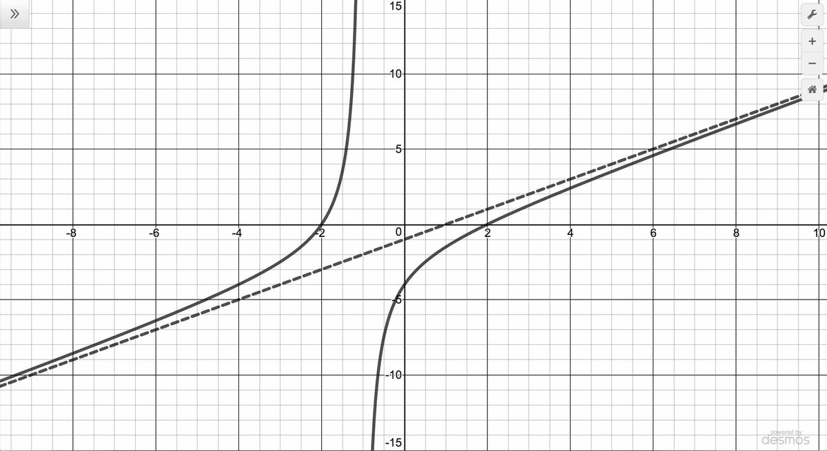
We close this section with a discussion of the third (and final!) kind of asymptote which can be associated with the graphs of rational functions. Let us return to the function in Example 3.1.6. Performing long division,20 we get . Since the term as and as , it stands to reason that as becomes unbounded, the function values . Geometrically, this means that the graph of should resemble the line as and . We see this play out both numerically and graphically below. (As usual, the asymptote is denoted by a dashed line.)
Table 3.1
Figure 3.31
The way we symbolize the relationship between the end behavior of with that of the line is to write `as and , ' in order to have some notational consistency with what we have done earlier in this section when it comes to end behavior.21 In this case, we say the line is a slant asymptote22 to the graph of . Informally, the graph of a rational function has a slant asymptote if, as or as , the graph resembles a non-horizontal, or `slanted' line. More formally, we define a slant asymptote as follows.
A few remarks are in order. First, note that the stipulation in Definition 3.6 is what makes the `slant' asymptote `slanted' as opposed to the case when in which case we'd have a horizontal asymptote.
Secondly, while we have motivated what me mean intuitively by the notation `,' like so many ideas in this section, the formal definition requires Calculus. Another way to express this sentiment, however, is to rephrase `' as `.' In other words, the graph of has the slant asymptote if and only if the graph of has a horizontal asymptote . This last sentiment can be encoded using limit notation as follows.
Our next task is to determine the conditions under which the graph of a rational function has a slant asymptote, and if it does, how to find it. In the case of , the degree of the numerator is , which is exactly one more than the degree if its denominator which is . This results in a linear quotient polynomial, and it is this quotient polynomial which is the slant asymptote. Generalizing this situation gives us the following theorem.23
In the same way that Theorem 3.3 gives us an easy way to see if the graph of a rational function has a horizontal asymptote by comparing the degrees of the numerator and denominator, Theorem 3.4 gives us an easy way to check for slant asymptotes. Unlike Theorem 3.3, which gives us a quick way to find the horizontal asymptotes (if any exist), Theorem 3.4 gives us no such `short-cut'. If a slant asymptote exists, we have no recourse but to use long division to find it.24
Our last example gives a real-world application of a slant asymptote. The problem features the concept of average profit. The average profit, denoted , is the total profit, , divided by the number of items sold, . In English, the average profit tells us the profit made per item sold. It, along with average cost, is defined below.
You'll explore average cost (and its relation to variable cost) in Exercise. For now, we refer the reader to to Example 1.4.3 in Section 1.4.
Exercises
(Review of Long Division):27 In Exercises -, use polynomial long division to perform the indicated division. Write the polynomial in the form .
In Exercises -, given the pair of functions and , sketch the graph of by starting with the graph of and using Theorem 3.1. Track at least two points and the asymptotes. State the domain and range using interval notation.
,
,
,
,
In Exercises -, find a formula for each function below in the form .
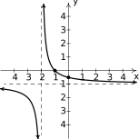
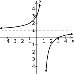
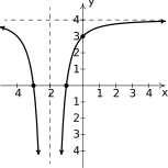
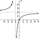
Figure 3.37-intercept , -intercept
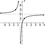
Figure 3.38-intercept , -intercept
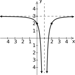
In Exercises -, find a formula for each function below in the form .
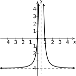
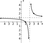
Figure 3.39-intercepts , , -intercept
Figure 3.40-intercepts , , Vertical Asymptote:
In Exercises -, for the given rational function:
State the domain.
Identify any vertical asymptotes of the graph.
Identify any holes in the graph.
Find the horizontal asymptote, if it exists.
Find the slant asymptote, if it exists.
Graph the function using a graphing utility and describe the behavior near the asymptotes.
The cost in dollars to remove % of the invasive Ippizuti fish species from Sasquatch Pond is:
Find and interpret and .
What does the vertical asymptote at mean within the context of the problem?
What percentage of the Ippizuti fish can you remove for $40000?
In the scenario of Example 3.1.3, , gives the height of a model rocket above the Moon's surface, in feet, seconds after liftoff. For each of the times listed below, find and simplify a the formula for the average velocity between and (see Definition 3.5) and use to find and interpret the instantaneous velocity of the rocket at (See Example 3.1.3).
The population of Sasquatch in Portage County years after the year 1803 is modeled by the function
Find and interpret the horizontal asymptote of the graph of and explain what it means.
The cost in dollars, to make dOpi media players is , . You may wish to review the concepts of fixed and variable costs introduced in Example 1.2.3 in Section 1.2.2.
Find a formula for the average cost .
Find and interpret and .
How many dOpis need to be produced so that the average cost per dOpi is ?
Find and interpret .
Interpret the behavior of as .
This exercise explores the relationships between fixed cost, variable cost, and average cost. The reader is encouraged to revisit Example 1.2.3 in Section 1.2.2 as needed. Suppose the cost in dollars to make items is given by where and are positive real numbers.
Show the fixed cost (the money spent even if no items are made) is .
Show the variable cost (the increase in cost per item made) is .
Find a formula for the average cost when making items, .
Show for all and, moreover, as .
Interpret both geometrically and in terms of fixed, variable, and average costs.
Suppose the price-demand function for a particular product is given by where is the number of items made and sold for dollars. Here, and . If the cost (in dollars) to make of these products is also a linear function , show that the graph of the average profit function has a slant asymptote with slope and interpret.
In Exercise in Section 2.1, we fit a few polynomial models to the following electric circuit data. The circuit was built with a variable resistor. For each of the following resistance values (measured in kilo-ohms, ), the corresponding power to the load (measured in milliwatts, ) is given below.28
Table 3.2
Resistance: ()
1.012
2.199
3.275
4.676
6.805
9.975
Power: ()
1.063
1.496
1.610
1.613
1.505
1.314
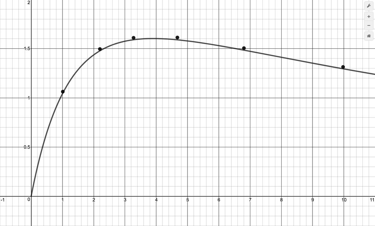
Using some fundamental laws of circuit analysis mixed with a healthy dose of algebra, we can derive the actual formula relating power to resistance :
Graph the data along with the function using a graphing utility.
Use a graphing utility to approximate the maximum power that can be delivered to the load. What is the corresponding resistance value?
Find and interpret the end behavior of as .
Let . Find values for and so the graph of has a hole at .
Let .
Find values for and so the graph of has the horizontal asymptote .
Find values for and so the graph of has the slant asymptote .
Suppose is a polynomial function and is a real number. Define . Use the Factor Theorem, Theorem 2.8, to prove the graph of has a hole at .
For each function listed below, compute the average rate of change over the indicated interval.29 What trends do you observe? How do your answers manifest themselves graphically? How do you results compare with those of Exercise in Section 2.1?
In his now famous 1919 dissertation The Learning Curve Equation, Louis Leon Thurstone presents a rational function which models the number of words a person can type in four minutes as a function of the number of pages of practice one has completed.30 Using his original notation and original language, we have where is the predicted practice limit in terms of speed units, is pages written, is writing speed in terms of words in four minutes, is equivalent previous practice in terms of pages and is the rate of learning. In Figure 5 of the paper, he graphs a scatter plot and the curve . Discuss this equation with your classmates. How would you update the notation? Explain what the horizontal asymptote of the graph means. You should take some time to look at the original paper. Skip over the computations you don't understand yet and try to get a sense of the time and place in which the study was conducted.
Domain: Vertical asymptote:
, No holes in the graph Horizontal asymptote:
More specifically: as
More specifically: as
Domain: Vertical asymptote:
, No holes in the graph Horizontal asymptote:
More specifically: as
More specifically: as
Domain: Vertical asymptotes:
,
, No holes in the graph Horizontal asymptote:
More specifically, as
More specifically, as
Domain: No vertical asymptotes No holes in the graph Horizontal asymptote:
More specifically, as
More specifically, as
Domain: Vertical asymptote:
No holes in the graph Horizontal asymptote:
31More specifically, as
More specifically, as
Domain: Vertical asymptote:
, Hole at Slant asymptote:
As , the graph is below
As , the graph is above
Domain: No vertical asymptotes No holes in the graph Horizontal asymptote:
More specifically, as
More specifically, as
Domain: Vertical asymptotes:
,
, No holes in the graph Horizontal asymptote:
More specifically, as
More specifically, as
Domain: Vertical asymptote:
, Hole at Horizontal asymptote:
More specifically, as
More specifically, as
Domain: Vertical asymptotes:
,
, No holes in the graph Horizontal asymptote:
More specifically, as
More specifically, as
Domain: Vertical asymptote:
, Hole at Slant asymptote:
As , the graph is below
As , the graph is above
Domain: No vertical asymptotes No holes in the graph Slant asymptote:
As , the graph is above
As , the graph is below
Domain: Vertical asymptote:
, No holes in the graph Slant asymptote:
As , the graph is above
As , the graph is below
Domain: Vertical asymptotes: ,
,
, No holes in the graph Slant asymptote:
As , the graph is above
As , the graph is below
Domain: Vertical asymptotes:
, No holes in the graph Slant asymptote:
As , the graph is above
As , the graph is below
Domain: Vertical asymptote:
No holes in the graph No horizontal or slant asymptote
Domain: No vertical asymptotes Holes in the graph at and Horizontal asymptote
Domain: No vertical asymptotes No holes in the graph Slant asymptote:
everywhere.
means it costs $590 to remove 25% of the fish and and means it would cost $33630 to remove 95% of the fish from the pond.
The vertical asymptote at means that as we try to remove 100% of the fish from the pond, the cost increases without bound; i.e., it's impossible to remove all of the fish.
For $40000 you could remove about 95.76% of the fish.
, . The instantaneous velocity of the rocket when is meaning it is traveling feet per second upwards.
, . The instantaneous velocity of the rocket when is , so the rocket has slowed to feet per second (but still heading up.)
, . The instantaneous velocity of the rocket when is , so the rocket has momentarily stopped! In Example 1.2.8, we learned the rocket reaches its maximum height when seconds, which means the rocket must change direction from heading up to coming back down, so it makes sense that for this instant, its velocity is .
, . The instantaneous velocity of the rocket when is meaning the rocket has, indeed, changed direction and is heading downwards at a rate of feet per second. (Note the symmetry here between this answer and our answer when .)
The horizontal asymptote of the graph of is and it means that the model predicts the population of Sasquatch in Portage County will never exceed 150.
, .
and . When just dOpi is produced, the cost per dOpi is , but when dOpis are produced, the cost per dOpi is .
when . So to get the cost per dOpi to , dOpis need to be produced.
We find . This means that as fewer and fewer dOpis are produced, the cost per dOpi becomes unbounded. In this situation, there is a fixed cost of (), we are trying to spread that over fewer and fewer dOpis.
As , . This means that as more and more dOpis are produced, the cost per dOpi approaches , but is always a little more than . Since is the variable cost per dOpi (), it means that no matter how many dOpis are produced, the average cost per dOpi will always be a bit higher than the variable cost to produce a dOpi. As before, we can attribute this to the fixed cost, which factors into the average cost per dOpi no matter how many dOpis are produced.
The cost to make items is . Hence, so the fixed costs are .
is a linear function with slope . Hence, the cost increases at a rate of dollars per item made. Hence, the variable cost is .
for .
Since , for . As , so .
Geometrically, the graph of has a horizontal asymptote , the variable cost. In terms of costs, as more items are produced, the affect of the fixed cost on the average cost, falls away so that the average cost per item approaches the variable cost to make each item.
If and is linear, say , then we can compute the the profit function (in general) as: which simplifies to . Hence, the average profit . We see that as , so . Hence, is the slant asymptote to . This means that as more items are sold, the average profit is decreasing at approximately the same rate as the price function is decreasing, dollars per item. That is, to sell one additional item, we drop the price by dollars which results in a drop in the average profit by approximately dollars.
Figure 3.45
The maximum power is approximately which corresponds to .
As which means as the resistance increases without bound, the power diminishes to zero.
and so .
and so
and so .
If we define then is a polynomial function with . The Factor Theorem guarantees is a factor of , that is, for some polynomial . Hence, so the graph of is the same as the graph of the polynomial except for a hole when .
The slope of the curves near matches the exponent on . This exactly what we saw in Exercise in Section 2.1.
Adapted from Precalculus with Integrated Calculus, edition 4i, by Carl Stitz and Jeff Zeager (stitz-zeager.com), licensed under CC BY-NC-SA 3.0. Changes were made: reformatted as an accessible XYZ web edition. License: CC-BY-NC-SA-3.0.
These eBooks are a prerelease and are not yet certified conformant with WCAG 2.1 AA or any other accessibility standard. Every page is built against an automated accessibility gate, and our target for the published editions is WCAG 2.2 Level AA. If something is unusable, please tell us.