2.2 The Remainder and Factor Theorems

In Section 2.1 we saw how much of the `local' behavior of the graph of a polynomial function is determined by the zeros of the polynomial function. In that section, the polynomial functions we were given were mostly, if not completely, factored which greatly simplified the process for determining zeros. In this section, we revisit the relationship between zeros and factors with the ultimate aim of taking a polynomial function given to us in the form stated in Definition 2.4 and determining its zeros.

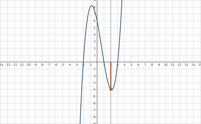
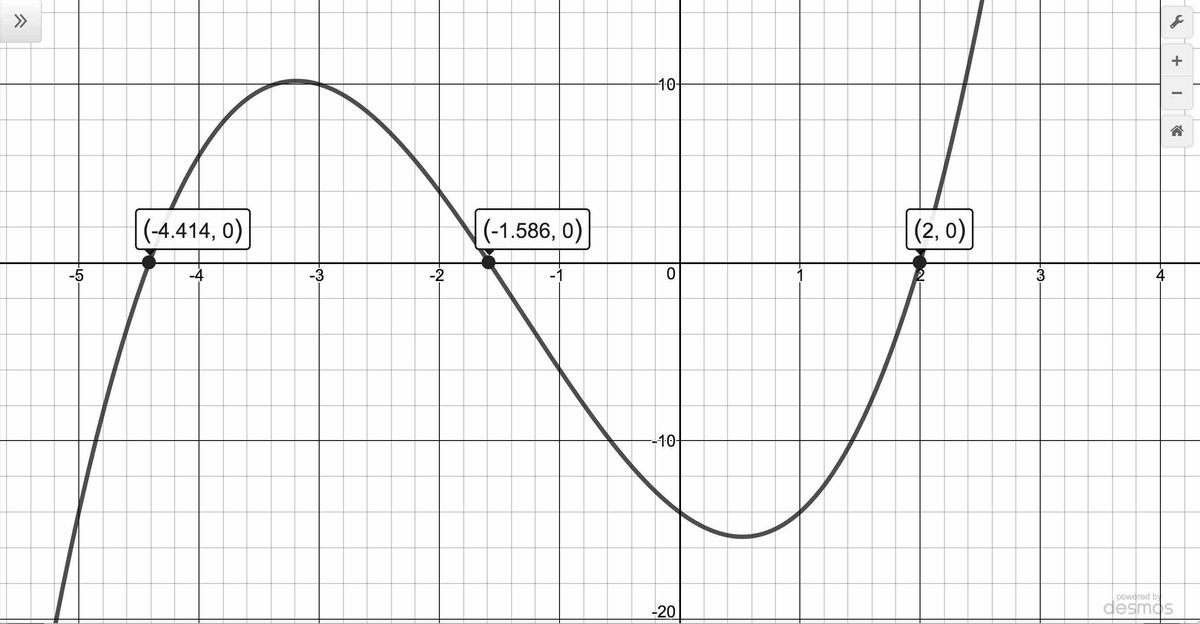
We start by way of example: suppose we wish to determine the zeros of $f (x) = x^{3} + 4 x^{2} - 5 x - 14$ . Setting $f ⁢ open parenthesis x close parenthesis equals 0$ results in the polynomial equation $x^{3} + 4 x^{2} - 5 x - 14 = 0$ . Despite all of the factoring techniques we learned (and forgot!) in Intermediate Algebra, this equation foils¹ us at every turn. Knowing that the zeros of $f$ correspond to $x$ -intercepts on the graph of $y = f (x)$ , we use a graphing utility to produce the graph below on the left.

The graph suggests that the function has three zeros, one of which appears to be $x equals 2$ and two others for whom we are provided what we assume to be decimal approximations: $x \approx - 4.414$ and $x \approx - 1.586$ . We can verify if these are zeros easily enough. We find $f (2) = {(2)}^{2} + 4 {(2)}^{2} - 5 (2) - 14 = 0$ , but $f (- 4.414) \approx 0.0039$ and $f (- 1.586) \approx 0.0022$ , While these last two values are probably by some measures, `close' to $0$ , they are not exactly equal to $0$ . The question becomes: is there a way to use the fact that $x equals 2$ is a zero to obtain the other two zeros?

Based on our experience, if $x equals 2$ is a zero, it seems that there should be a factor of $open parenthesis x minus 2 close parenthesis$ lurking around in the factorization of $f (x)$ . In other words, we should expect that $x^{3} + 4 x^{2} - 5 x - 14 = (x - 2) q (x)$ , where $q (x)$ is some other polynomial. How could we find such a $q (x)$ , if it even exists? The answer comes from our old friend, polynomial division. (See Section A.8.2.) Below on the right, we perform the long division: $(x^{3} + 4 x^{2} - 5 x - 14) \div (x - 2)$ and obtain $x^{2} + 6 x + 7$ .

$\begin{matrix} x^{2} & + & 6 x & + & 7 \\ x & - & 2 & x^{3} & + & 4 x^{2} & - & 5 x & - & 14 \\ - & (x^{3} & - & 2 x^{2}) \\ 6 x^{2} & - & 5 x \\ - & (6 x^{2} & - & 12 x) \\ 7 x & - & 14 \\ - & (7 x & - & 14) \\ 0 \end{matrix}$

Said differently, $f (x) = x^{3} + 4 x^{2} - 5 x - 14 = (x - 2) (x^{2} + 6 x + 7)$ . Using this form of $f (x)$ , we find the zeros by solving $(x - 2) (x^{2} + 6 x + 7) = 0$ . Setting each factor equal to $0$ , we get $x - 2 = 0$ (which gives us our known zero, $x equals 2$ ) as well as $x^{2} + 6 x + 7 = 0$ . The latter doesn't factor nicely, so we apply the Quadratic Formula to get $x = - 3 \pm \sqrt{2}$ . Sure enough, $- 3 - \sqrt{2} \approx - 4.414$ and $- 3 + \sqrt{2} \approx - 1.586$ . We leave it to the reader to show $f (- 3 - \sqrt{2}) = 0$ and $f (- 3 + \sqrt{2}) = 0$ . (See Exercise.)

The point of this section is to generalize the technique applied here. First up is a friendly reminder of what we can expect when we divide polynomials.

Theorem

Polynomial Division:

Suppose $d (x)$ and $p (x)$ are nonzero polynomial functions where the degree of $p$ is greater than or equal to the degree of $d$ . There exist two unique polynomial functions, $q (x)$ and $r (x)$ , such that $p (x) = d (x) q (x) + r (x),$ where either $r ⁢ open parenthesis x close parenthesis equals 0$ or the degree of $r$ is strictly less than the degree of $d$ .

As you may recall, all of the polynomials in Theorem 2.6 have special names. The polynomial $p$ is called the dividend; $d$ is the divisor; $q$ is the quotient; $r$ is the remainder. If $r ⁢ open parenthesis x close parenthesis equals 0$ then $d$ is called a factor of $p$ . The word `unique' here is critical in that it guarantees there is only one quotient and remainder for each division problem.² The proof of Theorem 2.6 is usually relegated to a course in Abstract Algebra, but we can still use the result to establish two important facts which are the basis of the rest of the chapter.

Theorem

The Remainder Theorem: Suppose $p$ is a polynomial function of degree at least $1$ and $c$ is a real number. When $p (x)$ is divided by $x - c$ the remainder is $p (c)$ . Said differently, there is a polynomial function $q (x)$ such that:

$p (x) = (x - c) q (x) + p (c)$

The proof of Theorem 2.7 is a direct consequence of Theorem 2.6. Since $x - c$ has degree $1$ , when a polynomial function is divided by $x - c$ , the remainder is either $0$ or degree $0$ (i.e., a nonzero constant.) In either case, $p (x) = (x - c) q (x) + r$ , where $r$ , the remainder, is a real number, possibly $0$ . It follows that $p (c) = (c - c) q (c) + r = 0 \cdot q (c) + r = r$ , so we get $r = p (c)$ as required. There is one last `low hanging fruit'³ to collect which we present below.

Once again, we see the phrase `if and only if' which means there are really two things being said in The Factor Theorem: if $(x - c)$ is a factor of $p (x)$ , then $c$ is a zero of $p$ and the only way $c$ is a zero of $p$ is if $(x - c)$ is a factor of $p (x)$ .

We argue the Factor Theorem as follows: if $(x - c)$ is a factor of $p (x)$ , then $p (x) = (x - c) q (x)$ for some polynomial $q$ . Hence, $p (c) = (c - c) q (c) = 0$ , so $c$ is a zero of $p$ . Conversely, suppose $c$ is a zero of $p$ , so $p ⁢ open parenthesis c close parenthesis equals 0$ . The Remainder Theorem tells us $p (x) = (x - c) q (x) + p (c) = (x - c) q (x) + 0 = (x - c) q (x)$ . Hence, $(x - c)$ is a factor of $p (x)$ .

We have enough theory to explain why the concept of multiplicity (Definition 2.6) is well-defined. If $c$ is a zero of $p$ , then The Factor Theorem tells us there is a polynomial function $q sub 1$ so that $p (x) = (x - c) q_{1} (x)$ . If $q sub 1 ⁢ open parenthesis c close parenthesis equals 0$ , then we apply the Factor Theorem to $q sub 1$ and find a polynomial $q sub 2$ so that $q_{1} (x) = (x - c) q_{2} (x)$ . Hence, we have

$p (x) = (x - c) q_{1} (x) = (x - c) (x - c) q_{2} (x) = {(x - c)}^{2} q_{2} (x) .$

We now `rinse and repeat' this process. Since the degree of $p$ is a finite number, this process has to end at some point. That is we arrive at a factorization $p (x) = {(x - c)}^{m} q (x)$ where $q ⁢ open parenthesis c close parenthesis not equal to 0$ . Suppose we arrive at a different factorization of $p$ using other methods. That is, we find $p (x) = {(x - c)}^{k} Q (x)$ , where $Q$ is a polynomial function with $Q ⁢ open parenthesis c close parenthesis not equal to 0$ . Then we have ${(x - c)}^{m} q (x) = {(x - c)}^{k} Q (x)$ .

If $m \neq k$ , then either $m < k$ or $m > k$ . If $m < k$ , then we may divide both sides by ${(x - c)}^{m}$ to get: $q (x) = {(x - c)}^{k - m} Q (x)$ . Since $k > m$ , $k minus m greater than 0$ and we would have $q (c) = {(c - c)}^{k - m} Q (c) = 0$ , a contradiction since we are assuming $q ⁢ open parenthesis c close parenthesis not equal to 0$ . The assumption that $m > k$ likewise ends in a contradiction. Therefore, we have $m = k$ , so $p (x) = {(x - c)}^{m} q (x) = {(x - c)}^{m} Q (x)$ . By the uniqueness guaranteed in Theorem 2.6, we must have that $q (x) = Q (x)$ . Hence, the number $m$ and quotient polynomial $q (x)$ are unique.

The process outlined above, in which we coax out factors of $p (x)$ one at a time until we have all of them serves as a template for our work to come. Of the things The Factor Theorem tells us, the most pragmatic is that we had better find a more efficient way to divide polynomial functions by quantities of the form $x - c$ . Fortunately, people like Ruffini and Horner have already blazed this trail. Let's take a closer look at the long division we performed at the beginning of the section and try to streamline it. First off, let's change all of the subtractions into additions by distributing through the $minus 1$ s.

$\begin{matrix} x^{2} & + & 6 x & + & 7 \\ x & - & 2 & x^{3} & + & 4 x^{2} & - & 5 x & - & 14 \\ - x^{3} & + & 2 x^{2} \\ 6 x^{2} & - & 5 x \\ - 6 x^{2} & + & 12 x \\ 7 x & - & 14 \\ - 7 x & + & 14 \\ 0 \end{matrix}$

Next, observe that the terms $- x^{3}$ , $minus 6 ⁢ x squared$ and $minus 7 ⁢ x$ are the exact opposite of the terms above them. The algorithm we use ensures this is always the case, so we can omit them without losing any information.

Also note that the terms we `bring down' (namely the $minus 5 ⁢ x$ and $minus 14$ ) aren't really necessary to recopy, so we omit them, too.

$\begin{matrix} x^{2} & + & 6 x & + & 7 \\ x & - & 2 & x^{3} & + & 4 x^{2} & - & 5 x & - & 14 \\ 2 x^{2} \\ 6 x^{2} \\ 12 x \\ 7 x \\ 14 \\ 0 \end{matrix}$

Let's move terms up a bit and copy the $x^{3}$ into the last row.

$\begin{matrix} x^{2} & + & 6 x & + & 7 \\ x & - & 2 & x^{3} & + & 4 x^{2} & - & 5 x & - & 14 \\ 2 x^{2} & 12 x & 14 \\ x^{3} & 6 x^{2} & 7 x & 0 \end{matrix}$

Note that by arranging things in this manner, each term in the last row is obtained by adding the two terms above it. Notice also that the quotient polynomial can be obtained by dividing each of the first three terms in the last row by $x$ and adding the results.

If you take the time to work back through the original division problem, you will find that this is exactly the way we determined the quotient polynomial. This means that we no longer need to write the quotient polynomial down, nor the $x$ in the divisor, to determine our answer.

$\begin{matrix} - 2 & x^{3} & + & 4 x^{2} & - & 5 x & - & 14 \\ 2 x^{2} & 12 x & 14 \\ x^{3} & 6 x^{2} & 7 x & 0 \end{matrix}$

We've streamlined things quite a bit so far, but we can still do more. Let's take a moment to remind ourselves where the $2 ⁢ x squared$ , $12 ⁢ x$ and $14$ came from in the second row. Each of these terms was obtained by multiplying the terms in the quotient, $x^{2}$ , $6 ⁢ x$ and $7$ , respectively, by the $minus 2$ in $x minus 2$ , then by $minus 1$ when we changed the subtraction to addition.

Multiplying by $minus 2$ then by $minus 1$ is the same as multiplying by $2$ , so we replace the $minus 2$ in the divisor by $2$ . Furthermore, the coefficients of the quotient polynomial match the coefficients of the first three terms in the last row, so we now take the plunge and write only the coefficients of the terms to get

$\begin{matrix} 2 & 1 & 4 & - 5 & - 14 \\ 2 & 12 & 14 \\ 1 & 6 & 7 & 0 \end{matrix}$

We have constructed a synthetic division tableau for this polynomial division problem. Let's re-work our division problem using this tableau to see how it greatly streamlines the division process.

To divide $x^{3} + 4 x^{2} - 5 x - 14$ by $x minus 2$ , we write $2$ in the place of the divisor and the coefficients of $x^{3} + 4 x^{2} - 5 x - 14$ in for the dividend. Then `bring down' the first coefficient of the dividend.

Table 2.3

\begin{matrix} 2 & 1 & 4 & - 5 & - 14 \end{matrix}

\begin{matrix} 2 & 1 & 4 & - 5 & - 14 \\ ↓ \\ 1 \end{matrix}

Next, take the $2$ from the divisor and multiply by the $1$ that was `brought down' to get $2$ . Write this underneath the $4$ , then add to get $6$ .

Table 2.4

\begin{matrix} 2 & 1 & 4 & - 5 & - 14 \\ ↓ & 2 \\ 1 \end{matrix}

\begin{matrix} 2 & 1 & 4 & - 5 & - 14 \\ ↓ & 2 \\ 1 & 6 \end{matrix}

Now take the $2$ from the divisor times the $6$ to get $12$ , and add it to the $minus 5$ to get $7$ .

Table 2.5

\begin{matrix} 2 & 1 & 4 & - 5 & - 14 \\ ↓ & 2 & 12 \\ 1 & 6 \end{matrix}

\begin{matrix} 2 & 1 & 4 & - 5 & - 14 \\ ↓ & 2 & 12 \\ 1 & 6 & 7 \end{matrix}

Finally, take the $2$ in the divisor times the $7$ to get $14$ , and add it to the $minus 14$ to get $0$ .

Table 2.6

\begin{matrix} 2 & 1 & 4 & - 5 & - 14 \\ ↓ & 2 & 12 & 14 \\ 1 & 6 & 7 \end{matrix}

\begin{matrix} 2 & 1 & 4 & - 5 & - 14 \\ ↓ & 2 & 12 & 14 \\ 1 & 6 & 7 & 0 \end{matrix}

The first three numbers in the last row of our tableau are the coefficients of the quotient polynomial. Remember, we started with a third degree polynomial and divided by a first degree polynomial, so the quotient is a second degree polynomial. Hence the quotient is $x^{2} + 6 x + 7$ .

The number in the box is the remainder. Synthetic division is our tool of choice for dividing polynomials by divisors of the form $x - c$ . It is important to note that it works only for these kinds of divisors.⁴

Also take note that when a polynomial (of degree at least $1$ ) is divided by $x - c$ , the result will be a polynomial of exactly one less degree. Finally, it is worth the time to trace each step in synthetic division back to its corresponding step in long division. While the authors have done their best to indicate where the algorithm comes from, there is no substitute for working through it yourself.

Example 1

Use synthetic division to perform the following polynomial divisions. Identify the quotient and remainder. Write the dividend, quotient and remainder in the form given in Theorem 2.6.

$(5 x^{3} - 2 x^{2} + 1) \div (x - 3)$
$(t^{3} + 8) \div (t + 2)$
$\frac{4 - 8 z - 12 z^{2}}{2 z - 3}$

When setting up the synthetic division tableau, the coefficients of even `missing' terms need to be accounted for, so we enter $0$ for the coefficient of $x$ in the dividend.
$3, 5, minus 2, 0, 1; ↓, 15, 39, 117; 5, 13, 39, 118$
Since the dividend was a third degree polynomial function, the quotient is a second degree (quadratic) polynomial function with coefficients $5$ , $13$ and $39$ : $q (x) = 5 x^{2} + 13 x + 39$ . The remainder is $r ⁢ open parenthesis x close parenthesis equals 118$ . According to Theorem 2.6, we have $5 x^{3} - 2 x^{2} + 1 = (x - 3) (5 x^{2} + 13 x + 39) + 118$ , which we leave to the reader to check.
To use synthetic division here, we rewrite $t plus 2$ as $t - (- 2)$ and proceed as before
$\begin{matrix} - 2 & 1 & 0 & 0 & 8 \\ ↓ & - 2 & 4 & - 8 \\ 1 & - 2 & 4 & 0 \end{matrix}$
We get the quotient $q (t) = t^{2} - 2 t + 4$ and the remainder $r ⁢ open parenthesis t close parenthesis equals 0$ . Relating the dividend, quotient and remainder gives: $t^{3} + 8 = (t + 2) (t^{2} - 2 t + 4)$ , which is a specific instance of the `sum of cubes' formula some of you may recall from Intermediate Algebra.
To divide $4 - 8 z - 12 z^{2}$ by $2 ⁢ z minus 3$ , two things must be done. First, we write the dividend in descending powers of $z$ as $- 12 z^{2} - 8 z + 4$ . Second, since synthetic division works only for factors of the form $z - c$ , we factor $2 ⁢ z minus 3$ as $2 (z - \frac{3}{2})$ . Hence, we are dividing $- 12 z^{2} - 8 z + 4$ by two factors: $2$ and $(z - \frac{3}{2})$ . Dividing first by $2$ , we obtain $- 6 z^{2} - 4 z + 2$ . Next, we divide $- 6 z^{2} - 4 z + 2$ by $(z - \frac{3}{2})$ :
$\begin{matrix} \frac{3}{2} & - 6 & - 4 & 2 \\ ↓ & - 9 & - \frac{39}{2} \\ - 6 & - 13 & - \frac{35}{2} \end{matrix}$
Hence, $- 6 z^{2} - 4 z + 2 = (z - \frac{3}{2}) (- 6 z - 13) - \frac{35}{2}$ . However when it comes to writing the dividend, quotient and remainder in the form given in Theorem 2.6, we need to find $q (z)$ and $r (z)$ so that $- 12 z^{2} - 8 z + 4 = (2 z - 3) q (z) + r (z)$ . Hence, starting with $- 6 z^{2} - 4 z + 2 = (z - \frac{3}{2}) (- 6 z - 13) - \frac{35}{2}$ , we multiply $2$ back on both sides:
$\begin{matrix} - 6 z^{2} - 4 z + 2 & = & (z - \frac{3}{2}) (- 6 z - 13) - \frac{35}{2} \\ 2 (- 6 z^{2} - 4 z + 2) & = & 2 [(z - \frac{3}{2}) (- 6 z - 13) - \frac{35}{2}] \\ - 12 z^{2} - 8 z + 4 & = & 2 (z - \frac{3}{2}) (- 6 z - 13) - 2 (\frac{35}{2}) \\ - 12 z^{2} - 8 z + 4 & = & (2 z - 3) (- 6 z - 13) - 35 \end{matrix}$
At this stage, we have written $- 12 z^{2} - 8 z + 4$ in the form $(2 z - 3) q (z) + r (z)$ , so we identify the quotient as $q (z) = - 6 z - 13$ and the remainder is $r (z) = - 35$ .
But how can we be sure these are the same quotient and remainder polynomial functions we would have obtained if we had taken the time to do the long division in the first place? Because of the word `unique' in Theorem 2.6. The theorem states that there is only one way to decompose $- 12 z^{2} - 8 z + 4$ as $(2 z - 3) q (z) + r (z)$ . Since we have found such a way, we can be sure it is the only way.⁵

The next example pulls together all of the concepts discussed in this section.

Example 2

Let $p (x) = 2 x^{3} - 5 x + 3$ .

Find $p ⁢ open parenthesis minus 2 close parenthesis$ using The Remainder Theorem. Check your answer by substitution.
Verify $x equals 1$ is a zero of $p$ and use this information to all the real zeros of $p$ .

The Remainder Theorem states $p ⁢ open parenthesis minus 2 close parenthesis$ is the remainder when $p (x)$ is divided by $x - (- 2)$ . We set up our synthetic division tableau below. We are careful to record the coefficient of $x^{2}$ as $0$ :
$\begin{matrix} - 2 & 2 & 0 & - 5 & 3 \\ ↓ & - 4 & 8 & - 6 \\ 2 & - 4 & 3 & - 3 \end{matrix}$
According to the Remainder Theorem, $p (- 2) = - 3$ . We can check this by direct substitution into the formula for $p (x)$ : $p (- 2) = 2 {(- 2)}^{3} - 5 (- 2) + 3 = - 16 + 10 + 3 = - 3$ .
We verify $x equals 1$ is a zero of $p$ by evaluating $p (1) = 2 {(1)}^{3} - 5 (1) + 3 = 0$ . To see if there are any more real zeros, we need to solve $p (x) = 2 x^{3} - 5 x + 3 = 0$ . From the Factor Theorem, we know since $p ⁢ open parenthesis 1 close parenthesis equals 0$ , we can factor $p (x)$ as $open parenthesis x minus 1 close parenthesis ⁢ q ⁢ open parenthesis x close parenthesis$ . To find $q (x)$ , we use synthetic division:
$\begin{matrix} 1 & 2 & 0 & - 5 & 3 \\ ↓ & 2 & 2 & - 3 \\ 2 & 2 & - 3 & 0 \end{matrix}$
As promised, our remainder is $0$ , and we get $p (x) = (x - 1) (2 x^{2} + 2 x - 3)$ . Setting this form of $p (x)$ equal to $0$ we get $(x - 1) (2 x^{2} + 2 x - 3) = 0$ . We recover $x equals 1$ from setting $x - 1 = 0$ but we also obtain $x = \frac{- 1 \pm \sqrt{7}}{2}$ from $2 x^{2} + 2 x - 3 = 0$ , courtesy of the Quadratic Formula.

Our next example demonstrates how we can extend the synthetic division tableau to accommodate zeros of multiplicity greater than $1$ .

Example 3

Let $p (x) = 4 x^{4} - 4 x^{3} - 11 x^{2} + 12 x - 3$ . Show $x = \frac{1}{2}$ is a zero of multiplicity $2$ and find all of the remaining real zeros of $p$ .

While computing $p (\frac{1}{2}) = 0$ shows $x = \frac{1}{2}$ is a zero of $p$ , to prove it has multiplicity $2$ , we need to factor $p (x) = {(x - \frac{1}{2})}^{2} q (x)$ with $q (\frac{1}{2}) \neq 0$ ,. We set up for synthetic division, but instead of stopping after the first division, we continue the tableau downwards and divide $(x - \frac{1}{2})$ directly into the quotient we obtained from the first division as follows:

$\begin{matrix} \frac{1}{2} & 4 & - 4 & - 11 & 12 & - 3 \\ ↓ & 2 & - 1 & - 6 & 3 \\ \frac{1}{2} & 4 & - 2 & - 12 & 6 & 0 \\ ↓ & 2 & 0 & - 6 \\ 4 & 0 & - 12 & 0 \end{matrix}$

We get:⁶ $4 x^{4} - 4 x^{3} - 11 x^{2} + 12 x - 3 = {(x - \frac{1}{2})}^{2} (4 x^{2} - 12)$ . Note if we let $q (x) = 4 x^{2} - 12$ , then $q (\frac{1}{2}) = 4 {(\frac{1}{2})}^{2} - 12 = - 11 \neq 0$ which proves $x = \frac{1}{2}$ is a zero of $p$ of multiplicity $2$ . To find the remaining zeros of $p$ , we set the quotient $4 x^{2} - 12 = 0$ , so $x squared equals 3$ and extract square roots to get $x = \pm \sqrt{3}$ .

A couple of things about the last example are worth mentioning. First, the extension of the synthetic division tableau for repeated divisions will be a common site in the sections to come. Typically, we will start with a higher order polynomial and peel off one zero at a time until we are left with a quadratic, whose roots can always be found using the Quadratic Formula.

Secondly, we found $x = \pm \sqrt{3}$ are zeros of $p$ . The Factor Theorem guarantees $(x - \sqrt{3})$ and $(x - (- \sqrt{3}))$ are both factors of $p$ . We can certainly put the Factor Theorem to the test and continue the synthetic division tableau from above to see what happens.

$\begin{matrix} \frac{1}{2} & 4 & - 4 & - 11 & 12 & - 3 \\ ↓ & 2 & - 1 & - 6 & 3 \\ \frac{1}{2} & 4 & - 2 & - 12 & 6 & 0 \\ ↓ & 2 & 0 & - 6 \\ \sqrt{3} & 4 & 0 & - 12 & 0 \\ ↓ & 4 \sqrt{3} & 12 \\ - \sqrt{3} & 4 & 4 \sqrt{3} & 0 \\ ↓ & - 4 \sqrt{3} \\ 4 & 0 \end{matrix}$

This gives us

$\begin{matrix} p (x) & = & 4 x^{4} - 4 x^{3} - 11 x^{2} + 12 x - 3 \\ = & {(x - \frac{1}{2})}^{2} (x - \sqrt{3}) (x - (- \sqrt{3})) (4) \\ = & 4 {(x - \frac{1}{2})}^{2} (x - \sqrt{3}) (x - (- \sqrt{3})) \end{matrix}$

We have shown that $p$ is a product of its leading coefficient times linear factors of the form $(x - c)$ where $c$ are zeros of $p$ . It may surprise and delight the reader that, in theory, all polynomials can be reduced to this kind of factorization. We leave that discussion to Section 2.4, because the zeros may not be real numbers. Our final theorem in the section gives us an upper bound on the number of real zeros.

Theorem 2.9 is a consequence of the Factor Theorem and polynomial multiplication. Every zero $c$ of $f$ gives us a factor of the form $(x - c)$ for $f (x)$ . Since $f$ has degree $n$ , there can be at most $n$ of these factors. The next section provides us some tools which not only help us determine where the real zeros are to be found, but which real numbers they may be.

We close this section with a summary of several concepts previously presented. You should take the time to look back through the text to see where each concept was first introduced and where each connection to the other concepts was made.

Connections Between Zeros, Factors and Graphs of Polynomial Functions

Suppose $p$ is a polynomial function of degree $n greater than or equal to 1$ . The following statements are equivalent:

The real number $c$ is a zero of $p$
$p ⁢ open parenthesis c close parenthesis equals 0$
$x = c$ is a solution to the polynomial equation $p ⁢ open parenthesis x close parenthesis equals 0$
$(x - c)$ is a factor of $p (x)$
The point $open parenthesis c, 0 close parenthesis$ is an $x$ -intercept of the graph of $y = p (x)$

Exercises

In Exercises -, use synthetic division to perform the following polynomial divisions. Identify the quotient and remainder. Write the divisor, quotient and remainder in the form given in Theorem 2.6.

$(3 x^{2} - 2 x + 1) \div (x - 1)$
$(x^{2} - 5) \div (x - 5)$
$(3 - 4 t - 2 t^{2}) \div (t + 1)$
$(4 t^{2} - 5 t + 3) \div (t + 3)$
$(z^{3} + 8) \div (z + 2)$
$(4 z^{3} + 2 z - 3) \div (z - 3)$
$(18 x^{2} - 15 x - 25) \div (x - \frac{5}{3})$
$(4 x^{2} - 1) \div (x - \frac{1}{2})$
$(2 t^{3} + t^{2} + 2 t + 1) \div (t + \frac{1}{2})$
$(3 t^{3} - t + 4) \div (t - \frac{2}{3})$
$(2 z^{3} - 3 z + 1) \div (z - \frac{1}{2})$
$(4 z^{4} - 12 z^{3} + 13 z^{2} - 12 z + 9) \div (z - \frac{3}{2})$
$(x^{4} - 6 x^{2} + 9) \div (x - \sqrt{3})$
$(x^{6} - 6 x^{4} + 12 x^{2} - 8) \div (x + \sqrt{2})$

In Exercises -, find $p (c)$ using the Remainder Theorem. If $p ⁢ open parenthesis c close parenthesis equals 0$ , use the Factor Theorem to partially factor the polynomial function.

$p (x) = 2 x^{2} - x + 1$ , $c equals 4$
$p (x) = 4 x^{2} - 33 x - 180$ , $c equals 12$
$p (t) = 2 t^{3} - t + 6$ , $c = - 3$
$p (t) = t^{3} + 2 t^{2} + 3 t + 4$ , $c = - 1$
$p (z) = 3 z^{3} - 6 z^{2} + 4 z - 8$ , $c equals 2$
$p (z) = 8 z^{3} + 12 z^{2} + 6 z + 1$ , $c = - \frac{1}{2}$
$p (x) = x^{4} - 2 x^{2} + 4$ , $c = \frac{3}{2}$
$p (x) = 6 x^{4} - x^{2} + 2$ , $c = - \frac{2}{3}$
$p (t) = t^{4} + t^{3} - 6 t^{2} - 7 t - 7$ , $c = - \sqrt{7}$
$p (t) = t^{2} - 4 t + 1$ , $c = 2 - \sqrt{3}$

In Exercises -, you are given a polynomial function and one of its zeros. Find the remaining real zeros and factor the polynomial.

$x^{3} - 6 x^{2} + 11 x - 6, c = 1$
$x^{3} - 24 x^{2} + 192 x - 512, c = 8$
$3 t^{3} + 4 t^{2} - t - 2, c = \frac{2}{3}$
$2 t^{3} - 3 t^{2} - 11 t + 6, c = \frac{1}{2}$
$z^{3} + 2 z^{2} - 3 z - 6, c = - 2$
$2 z^{3} - z^{2} - 10 z + 5, c = \frac{1}{2}$
$4 x^{4} - 28 x^{3} + 61 x^{2} - 42 x + 9$ , $c = \frac{1}{2}$ is a zero of multiplicity 2
$t^{5} + 2 t^{4} - 12 t^{3} - 38 t^{2} - 37 t - 12$ , $c = - 1$ is a zero of multiplicity 3
$125 z^{5} - 275 z^{4} - 2265 z^{3} - 3213 z^{2} - 1728 z - 324$ , $c = - \frac{3}{5}$ is a zero of multiplicity 3
$x^{2} - 2 x - 2, c = 1 - \sqrt{3}$
Find a quadratic polynomial with integer coefficients which has $x = \frac{3}{5} \pm \frac{\sqrt{29}}{5}$ as its real zeros.
For $f (x) = x^{3} + 4 x^{2} - 5 x - 14$ , show $f (- 3 - \sqrt{2}) = 0$ and $f (- 3 + \sqrt{2}) = 0$ two ways:
1. By direct substitution.
2. Using synthetic division and the Factor Theorem
Let $f (x) = a_{n} x^{n} + a_{n - 1} x^{n - 1} + \dots + a_{2} x^{2} + a_{1} x + a_{0}$ be a polynomial function with the property that $a_{n} + a_{n - 1} + \dots + a_{1} + a_{0} = 0$ . (That is, the sum of the coefficients and the constant term is $0$ .)
Prove that $open parenthesis x minus 1 close parenthesis$ is a factor of $f (x)$ .
HINT: Show $f ⁢ open parenthesis 1 close parenthesis equals 0$ and invoke the Factor Theorem
Verify the result in number with the functions: $f (x) = x^{3} - 2 x + 1$ and $f (x) = 3 x^{4} - x - 2$ .
Suppose $a$ is a nonzero real number. Find the quotients below, using synthetic division as required.
- $\frac{x - a}{x - a}$
- $\frac{x^{2} - a^{2}}{x - a}$
- $\frac{x^{3} - a^{3}}{x - a}$
- $\frac{x^{4} - a^{4}}{x - a}$
- $\frac{x^{5} - a^{5}}{x - a}$
Based on the pattern that evolves, find the quotient: $\frac{x^{10} - a^{10}}{x - a}$ . What about $\frac{x^{n} - a^{n}}{x - a}$ ?
Use your result from number to rewrite the sum: $1 + r + r^{2} + \dots + r^{n - 2} + r^{n - 1}$ as a quotient. What assumptions need to be made about $r$ ?

Answers

$(3 x^{2} - 2 x + 1) = (x - 1) (3 x + 1) + 2$
$(x^{2} - 5) = (x - 5) (x + 5) + 20$
$(3 - 4 t - 2 t^{2}) = (t + 1) (- 2 t - 2) + 5$
$(4 t^{2} - 5 t + 3) = (t + 3) (4 t - 17) + 54$
$(z^{3} + 8) = (z + 2) (z^{2} - 2 z + 4) + 0$
$(4 z^{3} + 2 z - 3) = (z - 3) (4 z^{2} + 12 z + 38) + 111$
$(18 x^{2} - 15 x - 25) = (x - \frac{5}{3}) (18 x + 15) + 0$
$(4 x^{2} - 1) = (x - \frac{1}{2}) (4 x + 2) + 0$
$(2 t^{3} + t^{2} + 2 t + 1) = (t + \frac{1}{2}) (2 t^{2} + 2) + 0$
$(3 t^{3} - t + 4) = (t - \frac{2}{3}) (3 t^{2} + 2 t + \frac{1}{3}) + \frac{38}{9}$
$(2 z^{3} - 3 z + 1) = (z - \frac{1}{2}) (2 z^{2} + z - \frac{5}{2}) - \frac{1}{4}$
$(4 z^{4} - 12 z^{3} + 13 z^{2} - 12 z + 9) = (z - \frac{3}{2}) (4 z^{3} - 6 z^{2} + 4 z - 6) + 0$
$(x^{4} - 6 x^{2} + 9) = (x - \sqrt{3}) (x^{3} + \sqrt{3} x^{2} - 3 x - 3 \sqrt{3}) + 0$
$(x^{6} - 6 x^{4} + 12 x^{2} - 8) = (x + \sqrt{2}) (x^{5} - \sqrt{2} x^{4} - 4 x^{3} + 4 \sqrt{2} x^{2} + 4 x - 4 \sqrt{2}) + 0$
$p ⁢ open parenthesis 4 close parenthesis equals 29$
$p ⁢ open parenthesis 12 close parenthesis equals 0$ , $p (x) = (x - 12) (4 x + 15)$
$p (- 3) = - 45$
$p (- 1) = 2$
$p ⁢ open parenthesis 2 close parenthesis equals 0$ , $p (z) = (z - 2) (3 z^{2} + 4)$
$p (- \frac{1}{2}) = 0$ , $p (z) = (z + \frac{1}{2}) (8 z^{2} + 8 z + 2)$
$p (\frac{3}{2}) = \frac{73}{16}$
$p (- \frac{2}{3}) = \frac{74}{27}$
$p (- \sqrt{7}) = 0$ , $p (t) = (t + \sqrt{7}) (t^{3} + (1 - \sqrt{7}) t^{2} + (1 - \sqrt{7}) t - \sqrt{7})$
$p (2 - \sqrt{3}) = 0$ , $p (t) = (t - (2 - \sqrt{3})) (t - (2 + \sqrt{3}))$
$x^{3} - 6 x^{2} + 11 x - 6 = (x - 1) (x - 2) (x - 3)$
$x^{3} - 24 x^{2} + 192 x - 512 = {(x - 8)}^{3}$
$3 t^{3} + 4 t^{2} - t - 2 = 3 (t - \frac{2}{3}) {(t + 1)}^{2}$
$2 t^{3} - 3 t^{2} - 11 t + 6 = 2 (t - \frac{1}{2}) (t + 2) (t - 3)$
$z^{3} + 2 z^{2} - 3 z - 6 = (z + 2) (z + \sqrt{3}) (z - \sqrt{3})$
$2 z^{3} - z^{2} - 10 z + 5 = 2 (z - \frac{1}{2}) (z + \sqrt{5}) (z - \sqrt{5})$
$4 x^{4} - 28 x^{3} + 61 x^{2} - 42 x + 9 = 4 {(x - \frac{1}{2})}^{2} {(x - 3)}^{2}$
$t^{5} + 2 t^{4} - 12 t^{3} - 38 t^{2} - 37 t - 12 = {(t + 1)}^{3} (t + 3) (t - 4)$
$125 z^{5} - 275 z^{4} - 2265 z^{3} - 3213 z^{2} - 1728 z - 324$ = $125 {(z + \frac{3}{5})}^{3} (z + 2) (z - 6)$
$x^{2} - 2 x - 2 = (x - (1 - \sqrt{3})) (x - (1 + \sqrt{3}))$
$p (x) = 5 x^{2} - 6 x - 4$
- For $f (x) = x^{3} - 2 x + 1$ , the coefficients $1 + (- 2) + 1 = 0$ and $f (x) = (x - 1) (x^{2} + x - 1)$ .
- For $f (x) = 3 x^{4} - x - 2$ the coefficients $3 + (- 1) + (- 2) = 0$ and $f (x) = (x - 1) (3 x^{3} + 3 x^{2} + 3 x + 2)$ .
- $\frac{x - a}{x - a} = 1$
- $\frac{x^{2} - a^{2}}{x - a} = x + a$
- $\frac{x^{3} - a^{3}}{x - a} = x^{2} + a x + a^{2}$
- $\frac{x^{4} - a^{4}}{x - a} = x^{3} + a x^{2} + a^{2} x + a^{3}$
- $\frac{x^{5} - a^{5}}{x - a} = x^{4} + a x^{3} + a^{2} x^{2} + a^{3} x + a^{4}$
Following the pattern:
- $\frac{x^{10} - a^{10}}{x - a} = x^{9} + a x^{8} + a^{2} x^{7} + a^{3} x^{6} + a^{4} x^{5} + a^{5} x^{4} + a^{6} x^{3} + a^{7} x^{2} + a^{8} x + a^{9}$
- $\frac{x^{n} - a^{n}}{x - a} = x^{n - 1} + a x^{n - 2} + a^{2} x^{n - 3} + \dots + a^{n - 2} x + a^{n - 1}$
Put $x equals 1$ and $a = r$ so that $1 + r + r^{2} + \dots + r^{n - 2} + r^{n - 1} = \frac{1 - r^{n}}{1 - r}$ . Here, $r not equal to 1$ as otherwise we'd be dividing by $0$ .

pun intended ↩
Hence the use of the definite article `the' when speaking of the quotient and the remainder. ↩
Jeff hates this expression and Carl included it just to annoy him. ↩
You'll need to use good old-fashioned polynomial long division for divisors of degree larger than 1. ↩
But it wouldn't hurt to check, just this once. ↩
For those wanting more detail: the first division gives: $4 x^{4} - 4 x^{3} - 11 x^{2} + 12 x - 3 = (x - \frac{1}{2}) (4 x^{3} - 2 x^{2} - 12 x + 6)$ . The second division gives: $4 x^{3} - 2 x^{2} - 12 x + 6 = (x - \frac{1}{2}) (4 x^{2} - 12)$ . ↩

Adapted from Precalculus, Preliminary 4th Edition (integrated calculus), by Carl Stitz and Jeff Zeager (stitz-zeager.com), licensed under CC BY-NC-SA 3.0. Changes were made: reformatted as an accessible XYZ web edition. License: CC-BY-NC-SA-3.0.