
2.1 Graphs of Polynomial Functions
In Chapter 1, we studied functions of the form (constant functions), , (linear functions), and , (quadratic functions). In each case, we learned how to construct graphs, find zeros, describe behavior, and use the functions in each family to model real-world phenomena. One might wonder about functions of the form , , or functions containing even higher powers of . These are the polynomial functions and are the subject of study in this chapter.1 As you may recall, polynomials are the result of adding monomials, so we begin our study of polynomial functions with monomial functions.
Monomial Functions
Monomial functions, by definition, contain the constant functions along with a two parameter family of functions, . We use as the default independent variable here with and as parameters. From Section A.1.2, we recall that the set is the set of natural numbers, so examples of monomial functions include , , and . Note that the function is not a monomial function. Even though for all nonzero values of , is undefined,2 and hence does not have a domain of .3
We begin our study of the graphs of polynomial functions by studying graphs of monomial functions. Starting with where is even, we investigate the cases , and at the top of the next page. Numerically, we see that if , becomes much smaller as increases whereas if or , becomes much larger as increases. These trends manifest themselves geometrically as the graph `flattening' for and `narrowing' for as increases.4
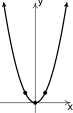
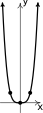
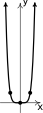
From the graphs, it appears as if the range of each of these functions is . When is even, for all so the range of is contained in . To show that the range of is all of , we note that the equation for has (at least) one solution for every even integer , namely . (See Section A.13 for a review of this notation.) Hence, which shows that every non-negative real number is in the range of .5
Another item worthy of note is the symmetry about the line a.k.a the -axis. (See Definition A.10 for a review of this concept.) With being even, . At the level of points, we have that for all , . Hence for every point on the graph of , the point symmetric about the -axis, is on the graph, too. We give this sort of symmetry a name honoring its roots here with even-powered monomial functions:
An investigation of the odd powered monomial functions () yields similar results with the major difference being that when a negative number is raised to an odd natural number power the result is still negative. Numerically we see that for the values of increase as increases and the values of get closer to as increases. This translates graphically into a flattening behavior on the interval and a narrowing elsewhere. The graphs are shown on the top of the next page.
The range of these functions appear to be all real numbers, which is algebraically sound as the equation has a solution for every real number,6 namely . Hence, for every real number , choose so that . This shows that every real number is in the range of .
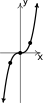
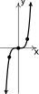
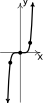
Here, since is odd, . This means that whenever is on the graph, so is the point symmetric about the origin, . (Again, see Definition A.10.) We generalize this property below. Not surprisingly, we name it in honor of its odd powered heritage:
The most important thing to take from the discussion above is the basic shape and common points on the graphs of for each of the families when even and is odd. While symmetry is nice and should be noted when present, even and odd symmetry are comparatively rare. The point of Definitions 2.2 and 2.3 is to give us the vocabulary to point out the symmetry when appropriate.
Moving on, we take a cue from Theorem 1.2 and prove the following.
Proof. Our goal is to start with the graph of and build it up to the graph of . We begin by examining . The graph of can be described as the set of points .7 Likewise, the graph of can be described as the set of points . If we relabel so that , then as varies through all real numbers so does .8 Hence, we can describe the graph of as . This means that we can obtain the graph of from the graph of by adding to each of the -coordinates of the points on the graph of and that establishes the first step of the theorem.
Next, we consider the graph of as compared to the graph of . The graph of is the set of points while the graph of is the set of points . The only difference between the points and is that the -coordinate in the latter is times the -coordinate of the former.
In other words, to produce the graph of from the graph of , we take the -coordinate of each point on the graph of and multiply it by to get the corresponding point on the graph of . If , all we are doing is scaling the -axis by . If , then, in addition to scaling the -axis, we are also reflecting each point across the -axis. In either case, we have established the second step of the theorem.
Last, we compare the graph of to that of . Once again, we view the graphs as sets of points in the plane. The graph of is and the graph of is. Looking at the corresponding points, and , we see that we can obtain all of the points on the graph of by adding to each of the -coordinates to points on the graph of . This is equivalent to shifting every point vertically by units which establishes the third and final step in the theorem.
This argument should sound familiar. The proof we presented above is more-or-less the same argument we presented after the proof of Theorem 1.2 in Section 1.3 but with `' replaced by `.' Also note that using in Theorem 2.1 establishes Theorem 1.3 in Section 1.4.
We now use Theorem 2.1 to graph two different “transformed” monomial functions. To provide the reader an opportunity to compare and contrast the graphical behaviors exhibited in the case when is even versus when is odd, we graph one of each case.
Example 2.1.1 demonstrates two big ideas in mathematics: first, resolving a complex problem into smaller, simpler steps, and, second, the value of changing form.9
Next we wish to focus on the so-called end behavior presented in each case.10 The end behavior of a function is a way to describe what is happening to the outputs from a function as the inputs approach the `ends' of the domain. Since domain of monomial functions is , we are looking to see what these functions do as their inputs `approach' and . The best we can do is sample inputs and outputs and infer general behavior from these observations. The good news is we've wrestled with this concept before. Indeed, every time we add `arrows' to the graph of a function, we've indicated its end behavior.11 Let's revisit the graph of using the table below.
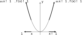
As takes on negative values that are larger in absolute value,12 we see takes on larger and larger positive values, seemingly without bound.13 It should be stressed that since `' and `' aren't real numbers, we can't write `,' so in order to communicate this behavior, we write as , , or, more succinctly, . Note that this latter notation is borrowed from Calculus and is read `the limit as approaches of is '.
Graphically, the farther to the left we select inputs on the -axis, the farther up the -axis the output (function) values are. We indicate this by attaching an `arrow' on the graph in Quadrant II indicating the graph continues to head upward to the left.
Similarly, observing the behavior of as , we get that since as the values increase without bound, so do the values. Graphically we indicate this by an arrow on the graph in Quadrant I heading upwards to the right. This behavior holds for all functions where is even.14
Repeating this investigation for for , we find as and . This trend holds for all functions where is odd.
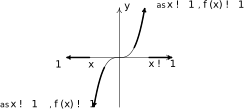
Theorem 2.2 summarizes the end behavior of monomial functions. The results are a consequence of Theorem 2.1 in that the end behavior of a function of the form only differs from that of if there is a reflection, that is, if .
Polynomial Functions
We are now in the position to discuss polynomial functions. Simply stated, polynomial functions are sums of monomial functions. The challenge becomes how to describe one of these beasts in general. Up until now, we have used distinct letters to indicate different parameters in our definitions of function families. In other words, we define constant functions as , linear functions as , and quadratic functions as . We even hinted at a function of the form . What happens if we wanted to describe a generic polynomial that required, say, 117 different parameters? Our work around is to use subscripted parameters, , that denote the coefficient of . For example, instead of writing a quadratic as , we describe it as , where , , and are real numbers and . As an added example, consider . We can re-write the formula for as and identify , , , , and . This is the notation we use in the following definition.
As usual, is used in Definition 2.4 as the independent variable with the each being a parameter. Even though we specify so , the value of the are unrestricted. Hence, any constant function can be written as , and so they are polynomials. Polynomials have an associated vocabulary,15 and hence, so do polynomial functions.
Again, constant functions are split off in their own separate case Definition 2.5 because of the ambiguity of . (See the remarks following Definition 2.1.) A consequence of Definition 2.5 is that we can now think of nonzero constant functions as `zeroth' degree polynomial functions, linear functions as `first' degree polynomial functions, and quadratic functions as `second' degree polynomial functions.
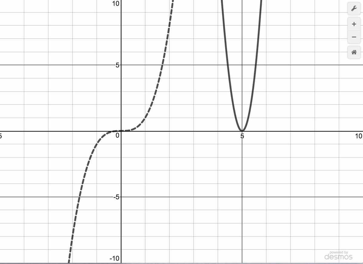
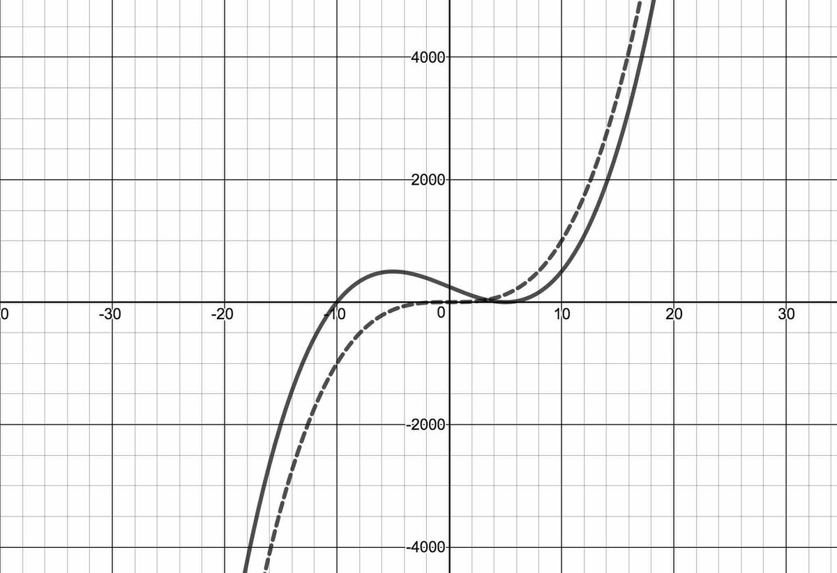
We now turn our attention to graphs of polynomial functions. Since polynomial functions are sums of monomial functions, it stands to reason that some of of the properties of those graphs carry over to more general polynomials. We first discuss end behavior. Consider . Below is the graph of (solid line) along with the graph of its leading term, (dashed line.) Below on the left is a view `near' the origin while below on the right is a `zoomed out' view. Near the origin, the graphs have little in common, but as we look farther out, it becomes that the functions begin to look quite similar.
and `near'
a `zoomed out' view
This observation is borne out numerically as well. Based on the table below, as or , it certainly appears as if . One way to think about what is happening numerically is that as or , the leading term dominates the lower order terms and . In other words, grows so much faster than and that these `lower order terms' don't contribute anything of significance to the so . To see this, we rewrite as17
As or , both and have constant numerators but denominators that are becoming unbounded. As such, both and . Therefore, as or ,
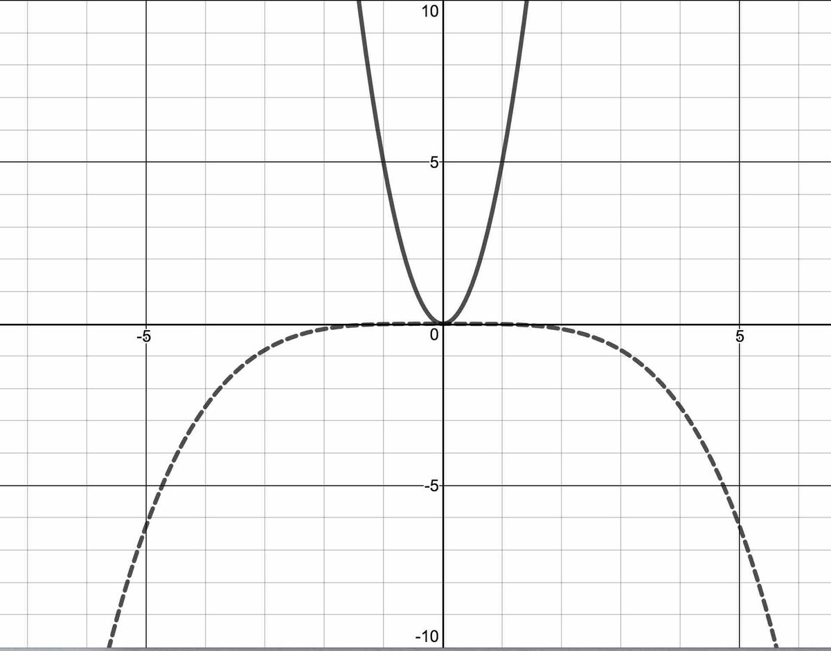
Next, consider . Following the logic of the above example, we would expect the end behavior of to mimic that of . When we graph (solid line) on the same set of axes as (dashed line), a view near the origin seems to suggest the exact opposite. However, zooming out reveals that the two graphs do share the same end behavior.18
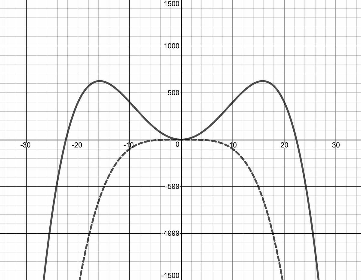
and `near'
a `zoomed out' view
Algebraically, for or , even with the small coefficient of , dominates the term so . More precisely,
The results of these last two examples generalize below in Theorem 2.3.
We argue Theorem 2.3 using an argument similar to ones used above. As or ,
If this argument looks a little fuzzy, it should. As with all things involving infinity, the precision of Calculus is required here19 For now, we'll rely on number sense and algebraic intuition.
Now that we know how to determine the end behavior of polynomial functions, it's time to investigate what happens `in between' the ends. First and foremost, polynomial functions are continuous. Recall from Section 1.4 that, informally, graphs of continuous functions have no `breaks' or `holes' in them.20 Since monomial functions are continuous (as far as we can tell) and polynomials are sums of monomial functions, it turns out that polynomial functions are continuous as well.
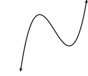
Moreover, the graphs of monomial functions, hence polynomial functions, are smooth. Once again, `smoothness' is a concept defined precisely in Calculus, but for us, functions have no `corners' or `sharp turns'. Below we find the graph of a function which is neither smooth nor continuous, and to its right we have a graph of a polynomial, for comparison.
The function whose graph appears on the left fails to be continuous where it has a `break' or `hole' in the graph; everywhere else, the function is continuous. The function is continuous at the `corner' and the `cusp', but we consider these `sharp turns', so these are places where the function fails to be smooth. Apart from these four places, the function is smooth and continuous. Polynomial functions are smooth and continuous everywhere, as exhibited in the graph on the right.
The notion of smoothness is what tells us graphically that, for example, , whose graph is the characteristic `' shape, cannot be a polynomial function, even though it is a piecewise-defined function comprised of polynomial functions. Knowing polynomial functions are continuous and smooth gives us an idea of how to `connect the dots' when sketching the graph from points that we're able to find analytically such as intercepts.
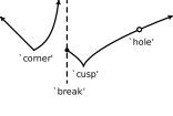
Pathologies not found on graphs of polynomials functions.
The graph of a polynomial function.
Speaking of intercepts, we next focus our attention on the behavior of the graphs of polynomial functions near their zeros. Recall a zero of a function is a solution to . Geometrically, the zeros of a function are the -coordinates of the -intercepts of the graph of .
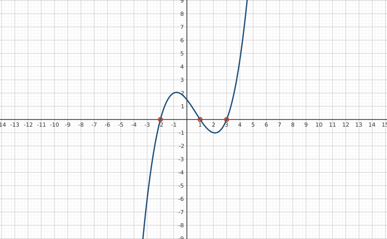
Consider the polynomial function . To find the zeros of , we set . Since the expression is already factored, we set each factor equal to zero.21
Solving gives , gives , and gives . Hence, our zeros are , , and .
Below, we graph and focus our attention near the -intercepts , and .
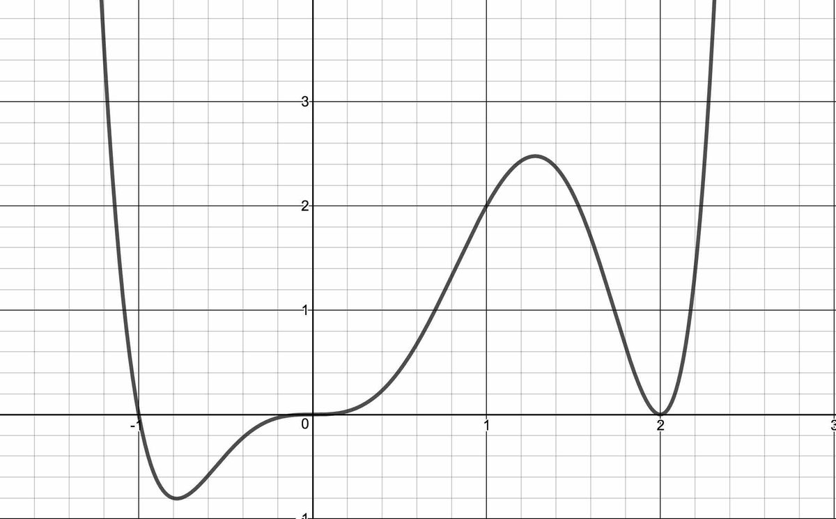
We first note that the graph crosses through the -axis at and , but the graph touches and rebounds at . Moreover, at , the graph crosses through the axis is a fairly `linear' fashion whereas there is a substantial amount of `flattening' going on near . Or aim is to explain these observations and generalize them.
First, let's look at what's happening with the formula when . We know the -intercept at is due to the presence of the factor in the expression for . So, in this sense, the factor is determining a major piece of the behavior of the graph near . For that reason, we focus instead on the other two factors to see what contribution they make.
We find when , and . Hence, . Below on the left is a graph of (the solid line) and the graph of (the dashed line.) Sure enough, these graphs approximate one another near .
Likewise, let's look near . The -intercept is due to the term. For , and , so . Below in the center picture, we have the graph of (again, the solid line) and (the dashed line) near . Once again, the graphs verify our analysis.
Last, but not least, we analyze near . Here, the intercept is due to the factor, so we look at the and factors. If , and . Hence, . Sure enough, as evidenced below on the right, the graphs of and .
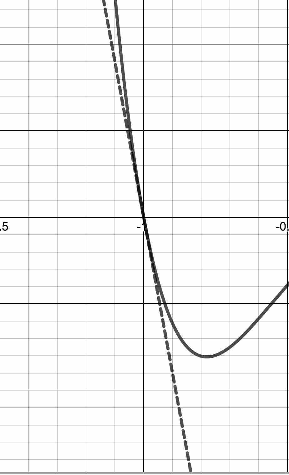
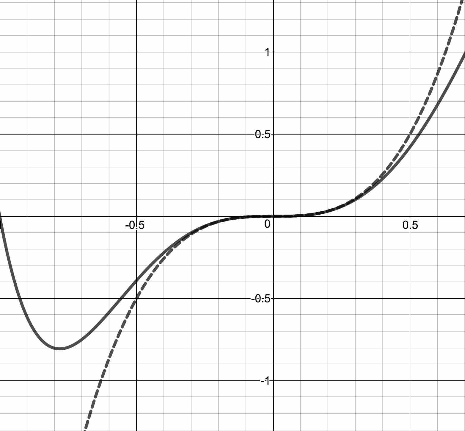
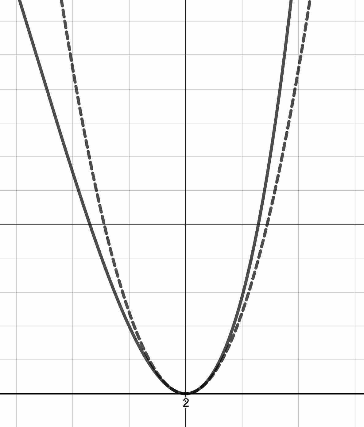
and
and
and
We generalize our observations in Theorem 2.4 below. Like many things we've seen in this text, a more precise statement and proof can be found in a course on Calculus.
Let's see how Theorem 2.4 applies to our findings regarding . For , . We rewrite and identify and . We find so Theorem 2.4 says that near , the graph of resembles .
For , and we can rewrite . We identify and . In this case , so Theorem 2.4 guarantees the graph of near resembles .
Lastly, for , we see and identify and . We find , so per Theorem 2.4, the graph of resembles near .
As we already mentioned, the formal statement and proof of Theorem 2.4 require Calculus. For now, we can understand the theorem as follows.
If we factor a polynomial function as where , then is a zero of , since . The stipulation that means that we have essentially factored the expression .
Thinking back to Theorem 2.1, the graph has an -intercept at , a basic overall shape determined by the exponent , and end behavior determined by the sign of .
The fact that if is a zero then we are guaranteed we can factor were and, moreover, such a factorization is unique (so that there's only one value of possible for each zero) is a consequence of two theorems, Theorem 2.6 and The Factor Theorem, Theorem 2.8 which we'll review in Section 2.2. For now, we assume such a factorization is unique in order to define the following.
So, for , is a zero of multiplicity , is a zero of multiplicity , and is a zero of multiplicity . Theorems 2.3 and 2.4 give us the following:
Our next example showcases how all of the above theory can assist in sketching relatively good graphs of polynomial functions without the assistance of technology.
A couple of remarks about Example 2.1.3 are in order. First, notice that the factor was more of a spectator in our discussion of the zeros of . Indeed, if we set , we have which provides no real solutions.22 That being said, the factor does affect the shape of the graph. 23
Next, when connecting up the graph from to to , there really is no way for us to know how low the graph goes, or where the lowest point is between and unless we plot more points. Likewise, we have no idea how high the graph gets between and . While there are ways to determine these points analytically, more often than not, finding them requires concepts from Calculus which we'll investigate later. Since these points do play an important role in many applications, we'll need to discuss them in this course and, when required, we'll use technology to find them. For that reason, we have the following definition:
Once again, the terminology used in Definition 2.7 blurs the line between the function and its outputs, . Also, some textbooks use the terms `relative' minimum and `relative' maximum instead of the adjective `local.' Lastly, note the definition of local extrema requires an open interval exist in the domain containing in order for to be a candidate for a local maximum or local minimum. We'll have more to say about this in later chapters. If our open interval happens to be , then our local extrema are the extrema of - we'll see an example of this momentarily.
Below we use a graphing utility to graph . We first consider the point . Even though there are points on the graph of that are higher than , locally, is the top of a hill. To satisfy Definition 2.7, we need to provide an open interval on which is the largest, or maximum function value. Note the definition requires us to provide just one open interval. One that works is the interval . We could use any smaller interval or go as large as .
Next we encounter a `low' point at approximately . More specifically, for all in the interval, say, , , Hence, we have a local minimum at . Lastly, at , we are back to a high point. In fact, isn't just a local maximum value, based on the graph, it is the maximum of . Here, we may choose the open interval as the open interval required by Definition 2.7, since for all , . It is important to note that there is no minimum value of despite there being a local minimum value.24
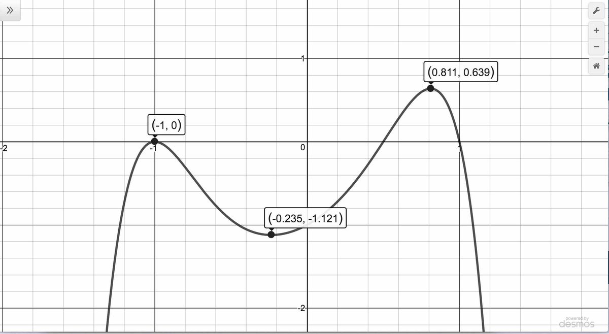
We close this section with a classic application of a third degree polynomial function.
Notice that there is a very slight, but important, difference between the function , from Example 2.1.4 and the function : their domains. The domain of is restricted to the interval while the domain of is . Indeed, the function has a maximum of (approximately) at (approximately) whereas for the function , is a local maximum value only. We leave it to the reader to verify that has neither a minimum nor a local minimum.
Exercises
In Exercises -, given the pair of functions and , sketch the graph of by starting with the graph of and using Theorem 2.1. Track at least three points of your choice through the transformations. State the domain and range of .
- ,
- ,
- ,
- ,
- ,
- ,
In Exercises -, find a formula for each function below in the form .
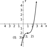
Figure 2.38 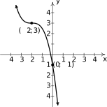
Figure 2.39
In Exercises -, find a formula for each function below in the form .
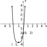
Figure 2.40 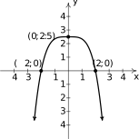
Figure 2.41
In Exercises -, find the degree, the leading term, the leading coefficient, the constant term and the end behavior of the given polynomial function.
In Exercises -, find the real zeros of the given polynomial and their corresponding multiplicities. Use this information along with end behavior to provide a rough sketch of the graph of the polynomial function. Compare your answer with the result from a graphing utility.
In Exercises -, determine analytically if the following functions are even, odd or neither. Confirm your answer using a graphing utility.
Suppose is a polynomial function written in the form of Definition 2.4.
- If the nonzero terms of consist of even powers of (or a constant), explain why is even.
- If the nonzero terms of consist of odd powers of , explain why is odd.
- If the nonzero terms of contain at least one odd power of and one even power of (or a constant term), then is neither even nor odd.
Use the results of Exercise to determine whether the following functions are even, odd, or neither.
- Show is an even function.
- Rework Example 2.1.4 assuming the box is to be made from an 8.5 inch by 11 inch sheet of paper. Using scissors and tape, construct the box. Are you surprised?26
For each function listed below, compute the average rate of change over the indicated interval.27 What trends do you observe? How do your answers manifest themselves graphically?
For each function listed below, compute the average rate of change over the indicated interval.28 What trends do you observe? How do your answers manifest themselves graphically?
In Exercises -, suppose the revenue , in thousands of dollars, from producing and selling hundred LCD TVs is given by for .
- Use a graphing utility to graph and determine the number of TVs which should be sold to maximize revenue. What is the maximum revenue?
Assume the cost, in thousands of dollars, to produce hundred LCD TVs is given by the function for . Find and simplify an expression for the profit function .
(Remember: Profit = Revenue - Cost.)
- Use a graphing utility to graph and determine the number of TVs which should be sold to maximize profit. What is the maximum profit?
- While developing their newest game, Sasquatch Attack!, the makers of the PortaBoy (from Example 1.2.3) revised their cost function and now use , for . As before, is the cost to make PortaBoy Game Systems. Market research indicates that the demand function remains unchanged. Use a graphing utility to find the production level that maximizes the profit made by producing and selling PortaBoy game systems.
According to US Postal regulations, a rectangular shipping box must satisfy the following inequality: “Length + Girth 130 inches” for Parcel Post and “Length + Girth 108 inches” for other services.
Let's assume we have a closed rectangular box with a square face of side length as drawn below. The length is the longest side and is clearly labeled. The girth is the distance around the box in the other two dimensions so in our case it is the sum of the four sides of the square, .
- Assuming that we'll be mailing a box via Parcel Post where Length + Girth 130 inches, express the length of the box in terms of and then express the volume of the box in terms of .
- Find the dimensions of the box of maximum volume that can be shipped via Parcel Post.
- Repeat parts and if the box is shipped using “other services”.
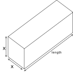
Figure 2.42 This exercise revisits the data set from Exercise in Section 1.4. In that exercise, you were given a chart of the number of hours of daylight they get on the of each month in Fairbanks, Alaska based on the 2009 sunrise and sunset data found on the U.S. Naval Observatory website. Here represents January 21, 2009, represents February 21, 2009, and so on.
Table 2.1 Month Number 1 2 3 4 5 6 7 8 9 10 11 12 Hours of Daylight 5.8 9.3 12.4 15.9 19.4 21.8 19.4 15.6 12.4 9.1 5.6 3.3 - Find cubic (third degree) and quartic (fourth degree) polynomials which model this data and comment on the goodness of fit for each. What can we say about using either model to make predictions about the year 2020? (Hint: Think about the end behavior of polynomials.)
- Use the models to see how many hours of daylight they got on your birthday and then check the website to see how accurate the models are.
- Sasquatch are largely nocturnal, so what days of the year according to your models allow for at least 14 hours of darkness for field research on the elusive creatures?
An electric circuit is built with a variable resistor installed. For each of the following resistance values (measured in kilo-ohms, ), the corresponding power to the load (measured in milliwatts, ) is given in the table below. 29
Table 2.2 Resistance: () 1.012 2.199 3.275 4.676 6.805 9.975 Power: () 1.063 1.496 1.610 1.613 1.505 1.314 - Make a scatter diagram of the data using the Resistance as the independent variable and Power as the dependent variable.
- Use your calculator to find quadratic (2nd degree), cubic (3rd degree) and quartic (4th degree) regression models for the data and judge the reasonableness of each.
- For each of the models found above, find the predicted maximum power that can be delivered to the load. What is the corresponding resistance value?
- Discuss with your classmates the limitations of these models - in particular, discuss the end behavior of each.
Below is a graph of a polynomial function as generated by a graphing utility. Answer the following questions about based on the graph provided.
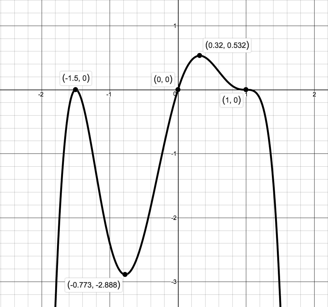
Figure 2.43 - Describe the end behavior of .
- List the real zeros of along with their respective multiplicities.
- List the local minimums and local maximums of the graph of .
- What can be said about the degree of and leading coefficient ?
- It turns out that is a seventh degree polynomial.30 How can this be?
- (This Exercise is a follow up to Example 2.1.3.) Use a graphing utility to compare and contrast the graphs of and .
- Use the graph of on page to estimate the largest open interval containing which satisfies the the criteria for `local minimum' in Definition 2.7.
- In light of Definition 2.7, explain why every point on the graph of a constant function is both a local maximum and a local minimum.
- This exercise involves the greatest integer function, , introduced in Example 1.2.2. Explain why the points for integers are local maximums but not local minimums.
- Use Theorems 2.3 and 2.4 prove Theorem 2.5.
Here are a few other questions for you to discuss with your classmates.
- How many and how few local extrema could a polynomial of degree have?
- Could a polynomial have two local maxima but no local minima?
- If a polynomial has two local maxima and two local minima, can it be of odd degree? Can it be of even degree?
- Can a polynomial have local extrema without having any real zeros?
- Why must every polynomial of odd degree have at least one real zero?
- Can a polynomial have two distinct real zeros and no local extrema?
- Can an -intercept yield a local extrema? Can it yield an absolute extrema?
- If the -intercept yields an absolute minimum, what can we say about the degree of the polynomial and the sign of the leading coefficient?
(This is a follow-up to Exercises in Section 1.2 and in Section 1.4.) The Lagrange Interpolate function for four points: , , , where , , , and are four distinct real numbers is given by the formula:
- Choose four points with different -values and construct the Lagrange Interpolate for those points. Verify each of the points lies on the polynomial.
- Verify that, in general, , , , and .
- Find for the points , , and . What happens?
- Find for the points , , and . What happens?
- Generalize the formula for to five points. What's the pattern?
Answers
domain: range:
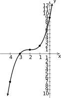
Figure 2.44 domain: range:
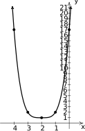
Figure 2.45 domain: range:
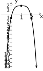
Figure 2.46 domain: range:
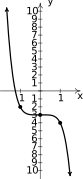
Figure 2.47 domain: range:
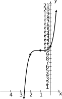
Figure 2.48 domain: range:
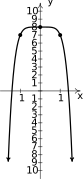
Figure 2.49 - Degree 2 Leading term Leading coefficient Constant term
- Degree 5 Leading term Leading coefficient Constant term
- Degree 4 Leading term Leading coefficient Constant term
- Degree 3 Leading term Leading coefficient Constant term
- Degree 17 Leading term Leading coefficient Constant term
- Degree 2 Leading term Leading coefficient Constant term
- Degree 4 Leading term Leading coefficient Constant term
- Degree 5 Leading term Leading coefficient Constant term
- Degree 6 Leading term Leading coefficient Constant term
- Degree 3 Leading term Leading coefficient Constant term
multiplicity 1 multiplicity 2

Figure 2.50 multiplicity 1 multiplicity 3
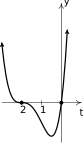
Figure 2.51 multiplicity 2 multiplicity 1
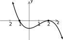
Figure 2.52 multiplicity 2 multiplicity 1
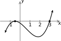
Figure 2.53 multiplicity 3 multiplicity 2

Figure 2.54 multiplicity 1 multiplicity 1 multiplicity 1 multiplicity 1
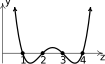
Figure 2.55 multiplicity 2 multiplicity 4
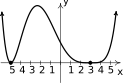
Figure 2.56 multiplicity 2 multiplicity 2 multiplicity 2
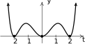
Figure 2.57 multiplicity 1
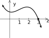
Figure 2.58 multiplicity 1 multiplicity 1 multiplicity 1
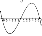
Figure 2.59 - odd
- neither
- even
- even
- even
- neither
- odd
- odd
- even
- odd
- neither
- even
- odd
- even
- even and odd
- even
- odd
- neither
- odd31
- For , . Hence, .
- , . Volume is maximized when , so we get the dimensions of the box with maximum volume are: height 1.58 inches, width 5.34 inches, and depth 7.84 inches. The maximum volume is 66.15 cubic inches.
Each of these average rates of change indicate slope of the curve over the given interval. Smaller slopes correspond to `flatter' curves and higher slopes correspond to `steeper' curves.
As we sample points closer to , the slope of the curve approaches the exponent on .
- The calculator gives the location of the absolute maximum (rounded to three decimal places) as and . Since represents the number of TVs sold in hundreds, corresponds to TVs. Since we can't sell half of a TV, we compare and , so selling TVs results in a (slightly) higher revenue. Since represents the revenue in thousands of dollars, the maximum revenue is .
- , .
- The calculator gives the location of the absolute maximum (rounded to three decimal places) as and . Since represents the number of TVs sold in hundreds, corresponds to TVs. Since we can't sell of a TV, we compare and , so selling TVs results in a (slightly) higher revenue. Since represents the revenue in thousands of dollars, the maximum revenue is .
- Making and selling 71 PortaBoys yields a maximized profit of $5910.67.
- To maximize the volume, we assume we start with the maximum Length Girth of , so the length is . The volume of a rectangular box is `length width height' so we get .
- Using a graphing utility, we get a (local) maximum of at . Hence, the maximum volume is using a box with dimensions .
- If we start with Length Girth then the length is so . Graphing shows a (local) maximum at so the dimensions of the box with maximum volume are for a volume of . (Calculus will confirm that the measurements which maximize the volume are exactly 18in. by 18in. by 36in., however, as I'm sure you are aware by now, we treat all numerical results as approximations and list them as such.)
- The cubic regression model is . It has which isn't bad. The graph of along with the data is shown below on the left. Note hits the -axis at about making this a bad model for future predictions.
- To use the model to approximate the number of hours of sunlight on your birthday, you'll have to figure out what decimal value of is close enough to your birthday and then plug it into the model. Jeff's birthday is July 31 which is 10 days after July 21 (). Assuming 30 days in a month, I think should work for my birthday and . The website says there will be about hours of daylight that day.
- To have 14 hours of darkness we need 10 hours of daylight. We see that and so it seems reasonable to say that we'll have at least 14 hours of darkness from December 21, 2008 () to February 21, 2009 () and then again from October 21,2009 () to December 21, 2009 ().
- The quartic regression model is . It has which is good. The graph of along with data is shown below on the right. Note is above making this a bad model as well for future predictions.
- Here, so this model more accurately predicts the number of hours of daylight on Jeff's birthday.
- This model says we'll have at least 14 hours of darkness from December 21, 2008 () to about March 1, 2009 () and then again from October 10, 2009 () to December 21, 2009 ().
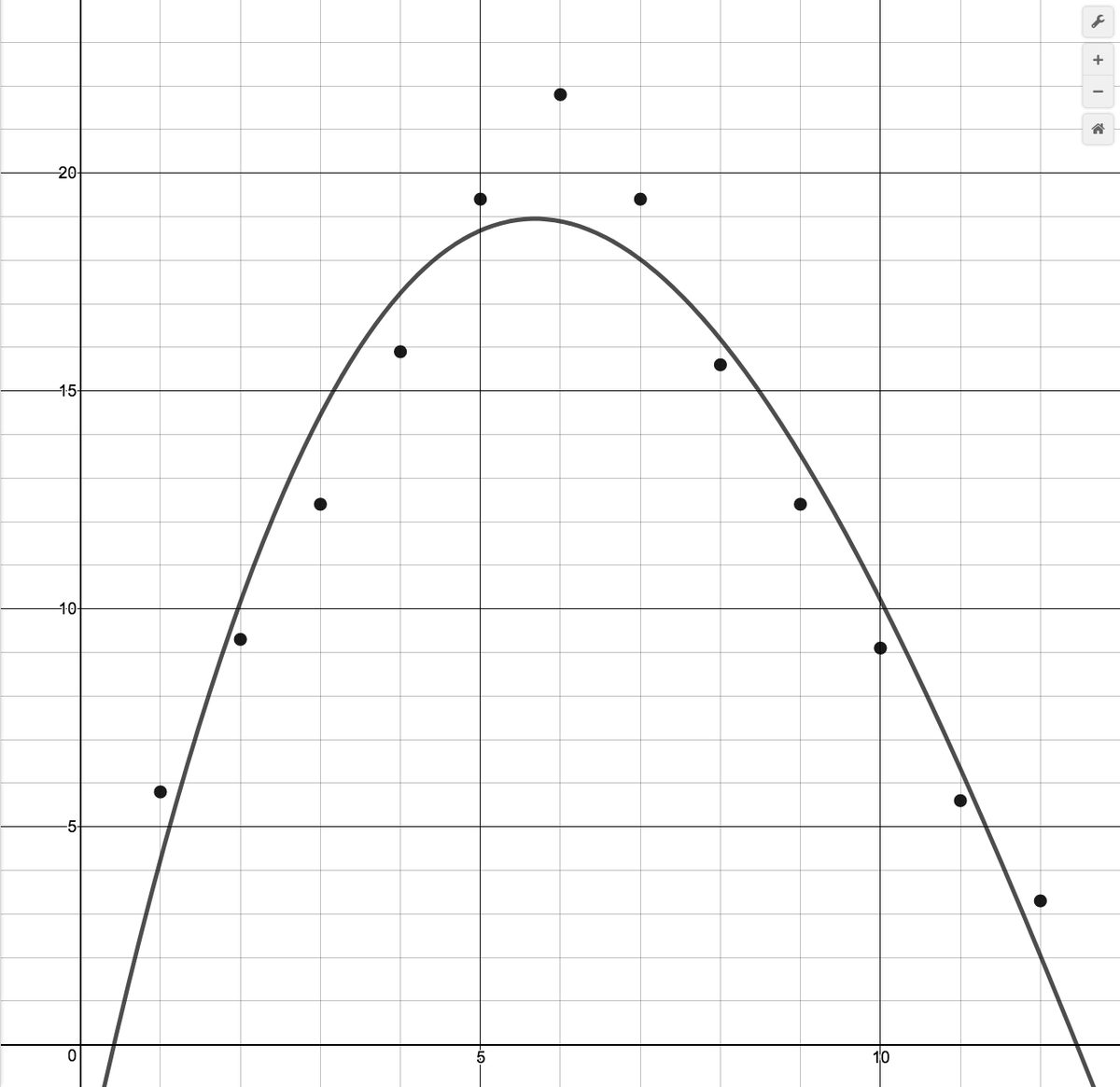
Figure 2.60 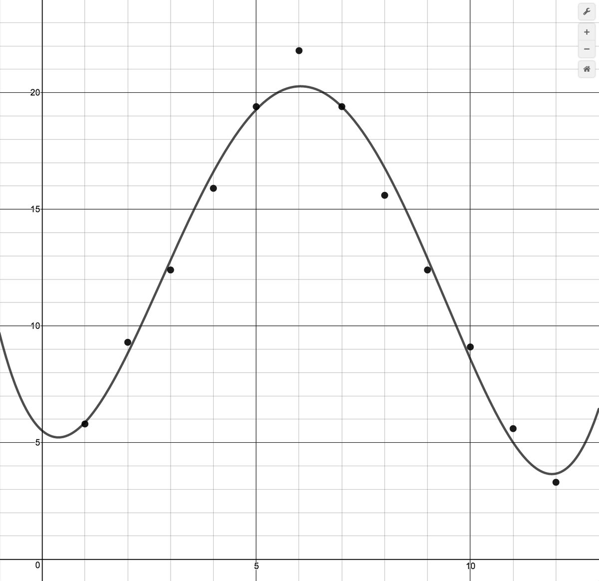
Figure 2.61 - The scatter plot is shown below with each of the three regression models.
- The quadratic model is , . The cubic model is , . The quartic model is , .
- The models give maximums: , and .
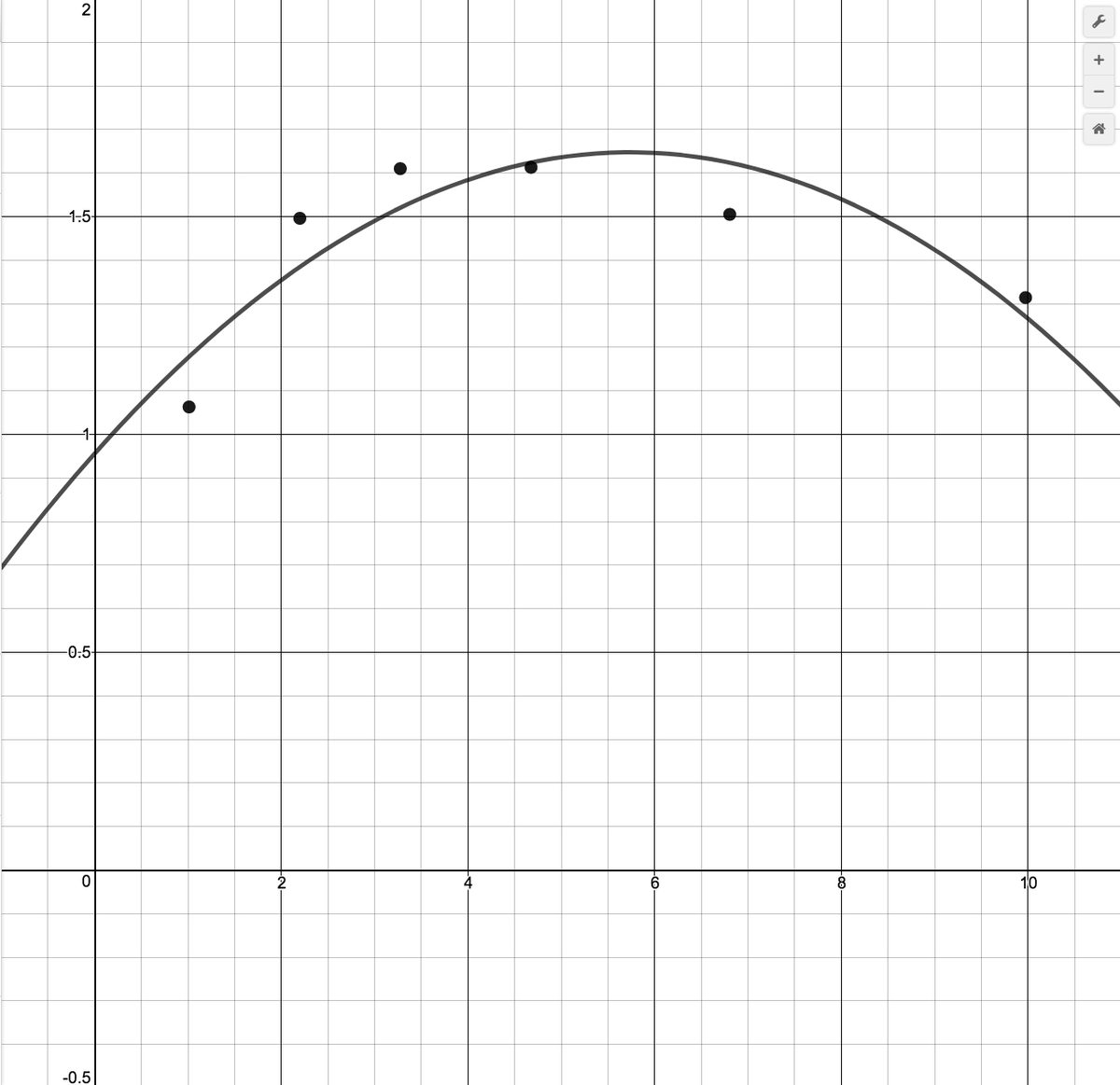
Figure 2.62 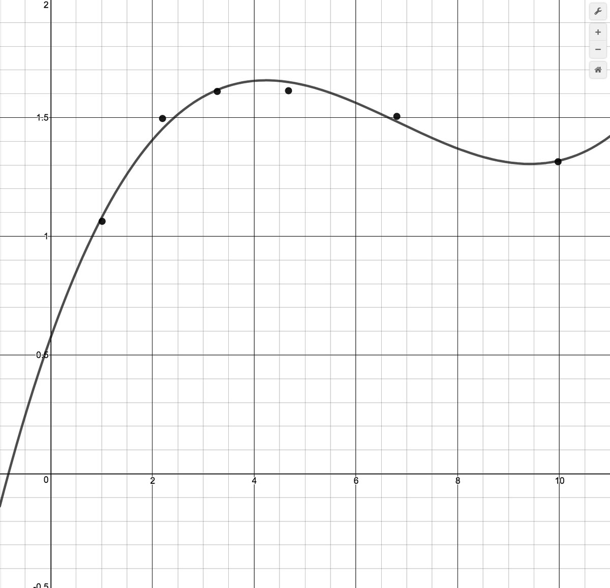
Figure 2.63 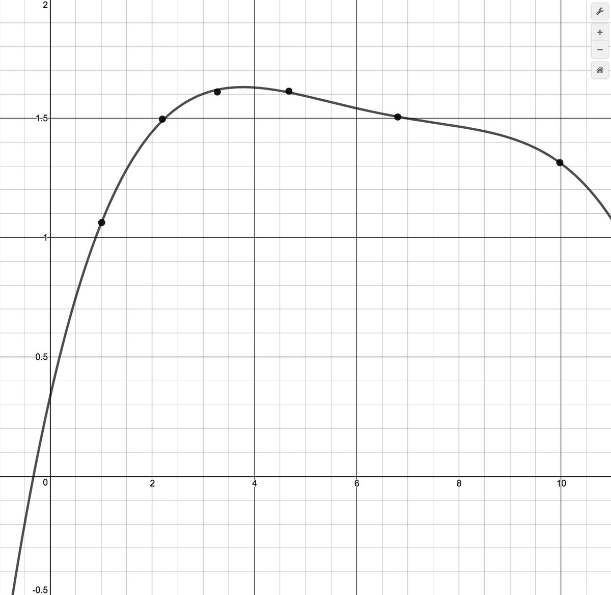
Figure 2.64 - and
- The zeros appear to be: , even multiplicity - probably since it doesn't `look like' the graph is very flat near ; , odd multiplicity - probably since the graph seems fairly linear as it passes through the origin; odd multiplicity - probably or higher since the graph seems fairly `flat' near .
- local minimum: approximately ; local maximums: approximately , and
- Based on the graph, even degree (at least based on multiplicities) with a negative leading coefficient based on the end behavior.
- We only have a portion of the graph represented here.
- We are looking for the largest open interval containing for which the graph of is at or above . Since each of the gridlines on the -axis correspond to units, we approximate this interval as .
Adapted from Precalculus with Integrated Calculus, edition 4i, by Carl Stitz and Jeff Zeager (stitz-zeager.com), licensed under CC BY-NC-SA 3.0. Changes were made: reformatted as an accessible XYZ web edition. License: CC-BY-NC-SA-3.0.