
1.4 Quadratic Functions
Graphs of Quadratic Functions
You may recall studying quadratic equations in a previous Algebra course. If not, you may wish to refer to Section A.10 to revisit this topic. In this section, we review those equations in the context of our next family of functions: the quadratic functions.
As in Definitions 1.4 and 1.5, the independent variable in Definition 1.10 is while the values , and are parameters. Note that - otherwise we would have a linear function (see Definition 1.5).
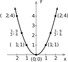
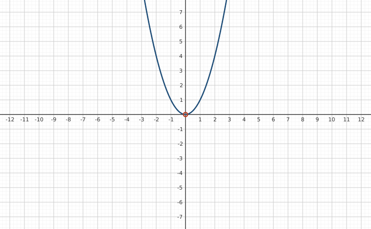
The most basic quadratic function is , the squaring function, whose graph appears below along with a corresponding table of values. Its shape may look familiar from your previous studies in Algebra – it is called a parabola. The point is called the vertex of the parabola because it is the sole point where the function obtains its extreme value, in this case, a minimum of when .
Indeed, the range of appears to be from the graph. We can substantiate this algebraically since for all , . This tells us that the range of is a subset of . To show that the range of actually equals , we need to show that every real number in is in the range of . That is, for every , we have to show is an output from . In other words, we have to show there is a real number so that . Choosing , we find , as required.1
The techniques we used to graph many of the absolute value functions in Section 1.3 can be applied to quadratic functions, too. In fact, knowing the graph of enables us to graph every quadratic function, but there's some extra work involved. We start with the following theorem:
To prove Theorem 1.3 the reader is encouraged to revisit the discussion following the proof of Theorem 1.2, replacing every occurrence of absolute value notation with the squared exponent.2 Alternatively, the reader can skip ahead and read the statement and proof of Theorem 2.1 in Section 2.1. In the meantime we put Theorem 1.3 to good use in the next example.
A few remarks about Example 1.4.1 are in order. First note that none of the functions are in the form of Definition 1.10. However, if we took the time to perform the indicated operations and simplify, we'd find:
While the -intercepts of the graphs of the each of the functions are easier to see when the formulas for the functions are written in the form of Definition 1.10, the vertex is not. For this reason, the form of the functions presented in Theorem 1.3 are given a special name.
If we proceed as in the remarks following Example 1.4.1, we can convert any quadratic function given to us in standard form and convert to general form by performing the indicated operation and simplifying:
With the identifications and , we have written in the form . Likewise, through a process known as `completing the square', we can take any quadratic function written in general form and rewrite it in standard form. We briefly review this technique in the following example – for a more thorough review the reader should see Section A.10.
We now generalize the procedure demonstrated in Example 1.4.2. Let for :
| [5pt] | Subtract from both sides. | ||
| [5pt] | Divide both sides by . | ||
| [10pt] | |||
| [10pt] | Add to both sides. | ||
| [10pt] | Factor the perfect square trinomial. | ||
| [10pt] | Solve for . | ||
| [10pt] | |||
| [10pt] | |||
| [10pt] | |||
| [10pt] | Get a common denominator. |
By setting and , we have written the function in the form . This establishes the fact that every quadratic function can be written in standard form.6 Moreover, writing a quadratic function in standard form allows us to identify the vertex rather quickly, and so our work also shows us that the vertex of is . It is not worth memorizing the expression especially since we can write this as . (This about this last statement for a moment.)
We summarize the information detailed above in the following:
Completing the square is also the means by which we may derive the celebrated Quadratic Formula, a formula which returns the solutions to for . Before we state it here for reference, we wish to encourage the reader to pause a moment and read the derivation if the Quadratic Formula found in Section A.10. The work presented in this section transforms the general form of a quadratic function into the standard form whereas the work in Section A.10 finds a formula to solve an equation. There is great value in understanding the similarities and differences between the two approaches.
It is worth pointing out the symmetry inherent in Equation 1.3. We may rewrite the zeros as:
so that, if there are real zeros, they (like the rest of the parabola) are symmetric about the line . Another way to view this symmetry is that the -coordinate of the vertex is the average of the zeros. We encourage the reader to verify this fact in all of the preceding examples, where applicable.
Next, recall that if the quantity is strictly negative then we do not have any real zeros. This quantity is called the discriminant and is useful in determining the number and nature of solutions to a quadratic equation. We remind the reader of this below.
We'll talk more about what we mean by a `repeated' zero and how to compute `non-real' zeros in Chapter 2. For us, the discriminant has the graphical implication that if then we have two -intercepts; if then we have just one -intercept, namely, the vertex; and if then we have no -intercepts because the parabola lies entirely above or below the -axis. We sketch each of these scenarios below assuming . (The sketches for are similar - see Exercise.)


We now revisit the economic scenario first described in Examples 1.2.3 and 1.2.4 where we were producing and selling PortaBoy game systems. Recall that the cost to produce PortaBoys is denoted by and the price-demand function, that is, the price to charge in order to sell systems is denoted by . We introduce two more related functions below: the revenue and profit functions.
Said differently, the revenue is the amount of money collected by selling items whereas the profit is how much money is left over after the costs are paid.
We hope Example 1.4.3 shows the value of using a continuous model to describe a discrete situation. True, we could have `run the numbers' and computed , , …, to eventually determine the maximum profit, but the vertex formula made much quicker work of the problem.
Along these same lines, in our next example we revisit Skippy's temperature data from Example 1.1.1 in Section 1.1. We found a piecewise-linear model in Section 1.2 to model the temperature over the course the day and now we seek a quadratic function to do the job. The methodology used here is similar to that of the least squares regression line discussed in Section 1.2.3 but instead of finding the line closest to the data points, we want the parabola closest to them that comes from a function of the form . The Mathematics required to find the desired quadratic function is beyond the scope of this text, but most graphing utilities can do these quickly. In the quadratic case, the machine will return a value of such that . The closer is to , the better the fit. (Again, how is computed is beyond this text.)
It is interesting how close the predictions from Examples 1.2.7 and 1.4.4 despite one using linear models and one using a quadratic model. Which model is the `better' model? We leave that discussion to the reader and their classmates.
Our next example is classic application of optimizing a quadratic function.
The function in Example 1.4.5 is called the objective function for this problem - it's the function we're trying to optimize. In the case above, we were trying to maximize . The equation along with the inequalities and are called the constraints. As we saw in this example, and as we'll see again and again, the constraint equation is used to rewrite the objective function in terms of just one of the variables where constraint inequalities, if any, help determine the applied domain.
Inequalities involving Quadratic Functions
We now turn our attention to solving inequalities involving quadratic functions. Consider the inequality . We could use the fact that the square root is increasing8 to get: , or . This reduces to or, using interval notation, . If, however, we had to solve , things are more complicated. One approach is to complete the square:
We get the solution . While there is nothing wrong with this approach, we seek methods here that will generalize to higher degree polynomials such as those we'll see in Chapter 2.
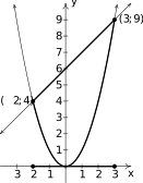
To that end, we look at the inequality graphically. Identifying and , we graph and on the same set of axes below on the left and look for where the graph of (the parabola) meets or is below the graph of (the line). There are two points of intersection which we determine by solving or . As usual, we rewrite this equation as in order to use the primary tools we've developed to handle these types9 of quadratic equations: factoring, or failing that, the Quadratic Formula. We find so we get two solutions to , namely and . Putting these together with the graph, we obtain the same solution: .
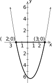
Yet a third way to attack is to rewrite the inequality as . Here, we graph to look for where the graph meets or is below the graph of , a.k.a. the -axis. Doing so requires us to find the zeros of , that is, solve from which we obtain and as before. We find the same solution, as is showcased in the graph at the bottom of the previous page on the right.
One advantage to using this last approach is that we are essentially concerned with one function and its zeros. This approach can be generalized to all functions - not just quadratics, so we take the time to develop this method more thoroughly now.
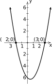
Consider the graph of below The zeros of are and and they divide the domain (the -axis) into three intervals: , and . For every number in , the graph of is above the -axis; in other words, for all in . Similarly, for all in , and for all in . We represent this schematically with the sign diagram below.
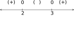
The above a portion of the number line indicates for those values of and the indicates there. The numbers labeled on the number line are the zeros of , so we place above them. For the inequality , we read from the sign diagram that the solution is .
Our next goal is to establish a procedure by which we can generate the sign diagram without graphing the function. While parabolas aren't that bad to graph knowing what we know, our sights are set on more general functions whose graphs are more complicated.
An important property of parabolas is that a parabola can't be above the -axis at one point and below the -axis at another point without crossing the -axis at some point in between. Said differently, if the function is positive at one point and negative at another, the function must have at least one zero in between. This property is a consequence of quadratic functions being continuous. A precise definition of `continuous' requires the language of Calculus, but it suffices for us to know that the graph of a continuous function has no gaps or holes. This allows us to determine the sign of all of the function values on a given interval by testing the function at just one value in the interval.
The result below applies to all continuous functions defined on an interval of real numbers, but we restrict our attention to quadratic functions for the time being,
Steps for Creating A Sign Diagram for A Quadratic Function
Suppose is a quadratic function.
- Find the zeros of and place them on the number line with the number above them.
- Choose a real number, called a test value, in each of the intervals determined in step 1.
- Determine and record the sign of for each test value in step 2.
To use a sign diagram to solve an inequality, we must always remember to compare the function to .
Solving Inequalities using Sign Diagrams
To solve an inequality using a sign diagram:
- Rewrite the inequality so some function is being compared to `.'
- Make a sign diagram for .
- Record the solution.
We practice this approach in the following example.
We end this section with an example that combines quadratic inequalities with piecewise functions.
Exercises
In Exercises -, graph the quadratic function. Find the vertex and axis intercepts of each graph, if they exist. State the domain and range, identify the maximum or minimum, and list the intervals over which the function is increasing or decreasing. If the function is given in general form, convert it into standard form; if it is given in standard form, convert it into general form.
In Exercises -, find a formula for each function below in the form .
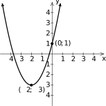
Figure 1.174 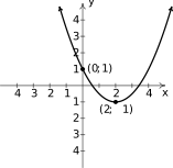
Figure 1.175 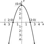
Figure 1.176 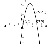
Figure 1.177
In Exercises - Find both the standard and general form of the quadratic functions below.
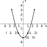
Figure 1.178 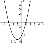
Figure 1.179 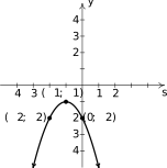
Figure 1.180 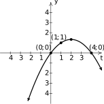
Figure 1.181
In Exercises -, solve the inequality. Write your answer using interval notation.
In Exercises -, cost and price-demand functions are given. For each scenario,
- Find the profit function .
- Find the number of items which need to be sold in order to maximize profit.
- Find the maximum profit.
- Find the price to charge per item in order to maximize profit.
- Find and interpret break-even points.
- The cost, in dollars, to produce “I'd rather be a Sasquatch” T-Shirts is , and the price-demand function, in dollars per shirt, is , for .
- The cost, in dollars, to produce bottles of All-Natural Certified Free-Trade Organic Sasquatch Tonic is , and the price-demand function, in dollars per bottle, is , for .
- The cost, in cents, to produce cups of Mountain Thunder Lemonade at Junior's Lemonade Stand is , and the price-demand function, in cents per cup, is , for .
- The daily cost, in dollars, to produce Sasquatch Berry Pies is , and the price-demand function, in dollars per pie, is , for .
- The monthly cost, in hundreds of dollars, to produce custom built electric scooters is , and the price-demand function, in hundreds of dollars per scooter, is , for .
- The International Silver Strings Submarine Band holds a bake sale each year to fund their trip to the National Sasquatch Convention. It has been determined that the cost in dollars of baking cookies is and that the demand function for their cookies is for . How many cookies should they bake in order to maximize their profit?
- Using data from Bureau of Transportation Statistics , the average fuel economy in miles per gallon for passenger cars in the US years after 1980 can be modeled by , . Find and interpret the coordinates of the vertex of the graph of .
The temperature , in degrees Fahrenheit, hours after 6 AM is given by:
What is the warmest temperature of the day? When does this happen?
- Suppose represents the costs, in hundreds, to produce thousand pens. How many pens should be produced to minimize the cost? What is this minimum cost?
- Skippy wishes to plant a vegetable garden along one side of his house. In his garage, he found 32 linear feet of fencing. Since one side of the garden will border the house, Skippy doesn't need fencing along that side. What are the dimensions of the garden which will maximize the area of the garden? What is the maximum area of the garden?
- In the situation of Example 1.4.5, Donnie has a nightmare that one of his alpaca fell into the river. To avoid this, he wants to move his rectangular pasture away from the river so that all four sides of the pasture require fencing. If the total amount of fencing available is still 200 linear feet, what dimensions maximize the area of the pasture now? What is the maximum area? Assuming an average alpaca requires 25 square feet of pasture, how many alpaca can he raise now?
- What is the largest rectangular area one can enclose with 14 inches of string?
- The height of an object dropped from the roof of an eight story building is modeled by by the function , . Here, is the height of the object off the ground, in feet, seconds after the object is dropped. How long before the object hits the ground?
- The height in feet of a model rocket above the ground seconds after lift-off is given by the function , for . When does the rocket reach its maximum height above the ground? What is its maximum height?
- Carl's friend Jason participates in the Highland Games. In one event, the hammer throw, the height in feet of the hammer above the ground seconds after Jason lets it go is modeled by the function . What is the hammer's maximum height? What is the hammer's total time in the air? Round your answers to two decimal places.
Assuming no air resistance or forces other than the Earth's gravity, the height above the ground at time of a falling object is given by where is in meters, is in seconds, is the object's initial velocity in meters per second and is its initial position in meters.
- What is the applied domain of this function?
- Discuss with your classmates what each of and would mean.
- Come up with a scenario in which .
- Let's say a slingshot is used to shoot a marble straight up from the ground with an initial velocity of 15 meters per second. What is the marble's maximum height above the ground? At what time will it hit the ground?
- If the marble is shot from the top of a 25 meter tall tower, when does it hit the ground?
- What would the height function be if instead of shooting the marble up off of the tower, you were to shoot it straight DOWN from the top of the tower?
- The two towers of a suspension bridge are 400 feet apart. The parabolic cable14 attached to the tops of the towers is 10 feet above the point on the bridge deck that is midway between the towers. If the towers are 100 feet tall, find the height of the cable directly above a point of the bridge deck that is 50 feet to the right of the left-hand tower.
On New Year's Day, Jeff started weighing himself every morning in order to have an interesting data set for this section of the book. (Discuss with your classmates if that makes him a nerd or a geek. Also, the professionals in the field of weight management strongly discourage weighing yourself every day. When you focus on the number and not your overall health, you tend to lose sight of your objectives. Jeff was making a noble sacrifice for science, but you should not try this at home.) The whole chart would be too big to put into the book neatly, so we've decided to give only a small portion of the data to you. This then becomes a Civics lesson in honesty, as you shall soon see. There are two charts given below. One has Jeff's weight for the first eight Thursdays of the year (January 1, 2009 was a Thursday and we'll count it as Day 1.) and the other has Jeff's weight for the first 10 Saturdays of the year.
Table 1.7 Day # (Thursday) 1 8 15 22 29 36 43 50 My weight in pounds 238.2 237.0 235.6 234.4 233.0 233.8 232.8 232.0 Table 1.8 Day # (Saturday) 3 10 17 24 31 38 45 52 59 66 My weight in pounds 238.4 235.8 235.0 234.2 236.2 236.2 235.2 233.2 236.8 238.2 - Find the least squares line for the Thursday data and comment on its goodness of fit.
- Find the least squares line for the Saturday data and comment on its goodness of fit.
- Use Quadratic Regression to find a parabola which models the Saturday data and comment on its goodness of fit.
- Compare and contrast the predictions the three models make for Jeff's weight on January 1, 2010 (Day #366). Can any of these models be used to make a prediction of Jeff's weight 20 years from now? Explain your answer.
- Why is this a Civics lesson in honesty? Well, compare the two linear models you obtained above. One was a good fit and the other was not, yet both came from careful selections of real data. In presenting the tables to you, we've not lied about Jeff's weight, nor have you used any bad math to falsify the predictions. The word we're looking for here is `disingenuous'. Look it up and then discuss the implications this type of data manipulation could have in a larger, more complex, politically motivated setting.
(Data that is neither linear nor quadratic.) We'll close this exercise set with two data sets that, for reasons presented later in the book, cannot be modeled correctly by lines or parabolas. It is a good exercise, though, to see what happens when you attempt to use a linear or quadratic model when it's not appropriate.
This first data set came from a Summer 2003 publication of the Portage County Animal Protective League called “Tattle Tails”. They make the following statement and then have a chart of data that supports it. “It doesn't take long for two cats to turn into 80 million. If two cats and their surviving offspring reproduced for ten years, you'd end up with 80,399,780 cats.” We assume .
Table 1.9 Year 1 2 3 4 5 6 7 8 9 10 Number of Cats 12 66 382 2201 12680 73041 420715 2423316 13968290 80399780 Use Quadratic Regression to find a parabola which models this data and comment on its goodness of fit. (Spoiler Alert: Does anyone know what type of function we need here?)
This next data set comes from the U.S. Naval Observatory . That site has loads of awesome stuff on it, but for this exercise I used the sunrise/sunset times in Fairbanks, Alaska for 2009 to give you a chart of the number of hours of daylight they get on the of each month. We'll let represent January 21, 2009, represent February 21, 2009, and so on.
Table 1.10 Month Number 1 2 3 4 5 6 7 8 9 10 11 12 Hours of Daylight 5.8 9.3 12.4 15.9 19.4 21.8 19.4 15.6 12.4 9.1 5.6 3.3 Use Quadratic Regression to find a parabola which models this data and comment on its goodness of fit. (Spoiler Alert: Does anyone know what type of function we need here?)
- Redraw the three scenarios discussed in the discriminant box for .
- Graph
- Find all of the points on the line which are units from .
- Let be the line . Find a function which measures the distance squared from a point on to . Use this to find the point on closest to .
- With the help of your classmates, show that if a quadratic function has two real zeros then the -coordinate of the vertex is the midpoint of the zeros.
On page, we argued that any quadratic function in standard form can be converted to a quadratic function in general form by making the identifications and . In this exercise, we use same identifications to show every parabola given in general form can be converted to standard form without completing the square.
Solve for and substitute the result into the equation and then solve for . Show and so that
In Exercises -, solve the quadratic equation for the indicated variable.
- for
- for
- for
- for
- for
- for (Assume .)
(This is a follow-up to Exercise in Section 1.2.) The Lagrange Interpolate function for three points , , and where , , and are three distinct real numbers is given by:
For each of the following sets of points, find using the formula above and verify each of the points lies on the graph of .
- , ,
- , ,
- , ,
- Verify that, in general, , , and .
- Find for the points , and . What happens?
- Under what conditions will produce a quadratic function? Make a conjecture, test some cases, and prove your answer.
Answers
(this is both forms!) No -intercepts -intercept Domain: Range: Decreasing on Increasing on Vertex is a minimum Axis of symmetry
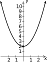
Figure 1.182 -intercept -intercept Domain: Range: Increasing on Decreasing on Vertex is a maximum Axis of symmetry
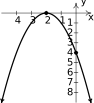
Figure 1.183 -intercepts and -intercept Domain: Range: Decreasing on Increasing on Vertex is a minimum Axis of symmetry
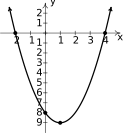
Figure 1.184 -intercepts and -intercept Domain: Range: Increasing on Decreasing on Vertex is a maximum Axis of symmetry
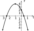
Figure 1.185 -intercepts and -intercept Domain: Range: Increasing on Decreasing on Vertex is a minimum Axis of symmetry
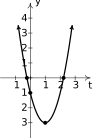
Figure 1.186 No -intercepts -intercept Domain: Range: Increasing on Decreasing on Vertex is a maximum Axis of symmetry
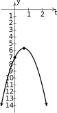
Figure 1.187 No -intercepts -intercept Domain: Range: Increasing on Decreasing on Vertex is a minimum Axis of symmetry
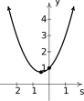
Figure 1.188 -intercepts and -intercept Domain: Range: Increasing on Decreasing on Vertex is a maximum Axis of symmetry
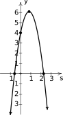
Figure 1.189 -intercepts and -intercept Domain: Range: Decreasing on Increasing on Vertex is a minimum15 Axis of symmetry
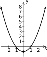
Figure 1.190 - No solution
- No solution
- , for .
- T-shirts should be made and sold to maximize profit.
- The maximum profit is .
- The price per T-shirt should be set at to maximize profit.
- The break even points are and , so to make a profit, between 1 and 13 T-shirts need to be made and sold.
- , for
- Since the vertex occurs at , and it is impossible to make or sell bottles of tonic, maximum profit occurs when either or bottles of tonic are made and sold.
- The maximum profit is .
- The price per bottle can be either (to sell 12 bottles) or (to sell 13 bottles.) Both will result in the maximum profit.
- The break even points are and , so to make a profit, between 5 and 20 bottles of tonic need to be made and sold.
- , for
- cups of lemonade need to be made and sold to maximize profit.
- The maximum profit is ¢ or .
- The price per cup should be set at ¢ per cup to maximize profit.
- The break even points are and , so to make a profit, between 4 and 20 cups of lemonade need to be made and sold.
- , for
- pies should be made and sold to maximize the daily profit.
- The maximum daily profit is .
- The price per pie should be set at to maximize profit.
- The break even points are and , so to make a profit, between 6 and 12 pies need to be made and sold daily.
- , for
- scooters need to be made and sold to maximize profit.
- The maximum monthly profit is hundred dollars, or .
- The price per scooter should be set at hundred dollars, or per scooter.
- The break even points are and , so to make a profit, between 10 and 50 scooters need to be made and sold monthly.
- 495 cookies
- The vertex is (approximately) , which corresponds to a maximum fuel economy of 22.66 miles per gallon, reached sometime between 2009 and 2010 (29 – 30 years after 1980.) Unfortunately, the model is only valid up until 2008 (28 years after 1908.) So, at this point, we are using the model to predict the maximum fuel economy.
- at 2 PM (8 hours after 6 AM.)
- 5000 pens should be produced for a cost of .
- 8 feet by 16 feet; maximum area is 128 square feet.
- 50 feet by 50 feet; maximum area is 2500 feet; he can raise 100 average alpacas.
- The largest rectangle has area square inches.
- seconds.
- The rocket reaches its maximum height of feet seconds after lift-off.
- The hammer reaches a maximum height of approximately feet. The hammer is in the air approximately seconds.
- The applied domain is .
- The height function is this case is . The vertex of this parabola is approximately so the maximum height reached by the marble is meters. It hits the ground again when seconds.
- The revised height function is which has zeros at and . We ignore the negative value and claim that the marble will hit the ground after seconds.
- Shooting down means the initial velocity is negative so the height functions becomes .
- Make the vertex of the parabola so that the point on the top of the left-hand tower where the cable connects is and the point on the top of the right-hand tower is . Then the parabola is given by . Standing feet to the right of the left-hand tower means you're standing at and . So the cable is 60.625 feet above the bridge deck there.
- The line for the Thursday data is . We have and so this is a really good fit.
- The line for the Saturday data is . We have and which is horrible. This data is not even close to linear.
- The parabola for the Saturday data is . We have which isn't good. Thus the data isn't modeled well by a quadratic function, either.
- The Thursday linear model had my weight on January 1, 2010 at 193.77 pounds. The Saturday models give 235.69 and 563.31 pounds, respectively. The Thursday line has my weight going below 0 pounds in about five and a half years, so that's no good. The quadratic has a positive leading coefficient which would mean unbounded weight gain for the rest of my life. The Saturday line, which mathematically does not fit the data at all, yields a plausible weight prediction in the end. I think this is why grown-ups talk about “Lies, Damned Lies and Statistics.”
- The quadratic model for the cats in Portage county is . Although this is not a good model because it's so far off for small values of . The model gives us 24,094,858 cats when but we know .
- The quadratic model for the hours of daylight in Fairbanks, Alaska is . Even with we should be wary of making predictions beyond the data. Case in point, the model gives hours of daylight when . So January 21, 2010 will be “extra dark”? Obviously a parabola pointing down isn't telling us the whole story.
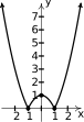
Figure 1.191 - ,
- is minimized when . Hence to find the point on closest to we substitute into to get .
- The three points lie on the same line and we get .
- To obtain a quadratic function, we require that the points are not collinear (i.e., they do not all lie on the same line.)
Adapted from Precalculus with Integrated Calculus, edition 4i, by Carl Stitz and Jeff Zeager (stitz-zeager.com), licensed under CC BY-NC-SA 3.0. Changes were made: reformatted as an accessible XYZ web edition. License: CC-BY-NC-SA-3.0.