
1.2 Constant and Linear Functions
Constant Functions
Now that we have defined the concept of a function, we'll spend the rest of Chapter 1 revisiting families of curves from prior courses in Algebra by viewing them through a `function lens'. We start with lines and refer the reader to Section A.5 for a review of the basic properties of lines. The simplest lines are vertical and horizontal lines. We leave it to the reader (see Exercise ) to think about why we eschew vertical lines in our discussion here, and begin with a functional description of horizontal lines.
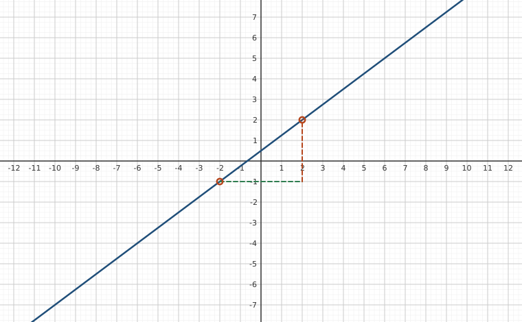
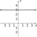
Consider the horizontal lines graphed in the -plane as shown below. The Vertical Line Test, Theorem 1.1, tells us that each describes as a function of so the question becomes how to represent these functions algebraically. The key here is to remember that the equation relating the independent variable , the dependent variable , and the function is given by .
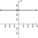
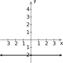
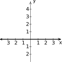
In the graph on the left, always equals so we have . Procedurally, `' says that the rule takes the input , and, regardless of that input, gives the output . This is an example of what is called a constant function - a function which returns the same value regardless of the input. Likewise, the function represented by the graph in the middle is , and the graph on the right (the -axis) is the graph of . In general, we have the following definition:
Some remarks about Definition 1.4 are in order. First, note that we are using `' as the independent variable, `' as the function name, and the letter `' as a parameter. In this context, a parameter is a fixed, but arbitrary, constant used to describe a family of functions. Different values of determine different constant functions. For example, gives , gives , and so on. Once is chosen, however, it does not change as the independent variable, , changes.
Also note that we are using the generic defaults for function names and independent variables, namely and , respectively. The functions and are also fine examples of constant functions. Recall that inherent in the definition of a function is the notion of domain, so we record (as part of the definition) that a constant function has domain . The range of a constant function is the set . The value in this case is both the maximum and minimum of , attained at each value in its domain.1
The next example showcases an application of constant functions and introduces the notion of a piecewise-defined function.
One of the favorite piecewise-defined functions in mathematical circles is the greatest integer of , denoted by . In Section we defined the set of integers as .4 The value is defined to be the largest integer with . That is, is the unique integer such that . Said differently, given any real number , if is an integer, then . If not, then lies in an interval between two integers, and and we choose , the left endpoint.
Linear Functions
Now that we've discussed the functions which correspond to horizontal lines, , we move to discussing the functions which can be represented by lines of the form where . These functions are called linear functions and are described below.
As with Definition 1.4, in Definition 1.5, is the independent variable, is the function name, and both and are parameters. Notice that is restricted by for if then the function would reduce to the constant function . The domain of linear functions, like that of constant functions, is specified as
Recall6 that the form of the line is called the slope-intercept form of the line and the slope, , and the -intercept , are easily determined when the line is written this way. Likewise, the form of the function in Definition 1.5, , is often called the slope-intercept form of a linear function.
The graph of a linear function is the graph of the line . Lines are uniquely determined by two points, and two points of geometric interest are the axis intercepts. We've already reminded you of the -intercept, , which is obtained by setting . Similarly, to find the -intercept, we set and solve for . We leave this to the reader in Exercise. In addition to having special graphical significance, axis intercepts quite often play important roles in applications involving both linear and non-linear functions. For that reason, we take the time to define them here using function notation.
As is customary in this text, Definition 1.6 uses the default independent variable , function name , and dependent variable , so these letters will change depending on the context. Also note that the `zeros' of a function are the solutions to - so they are real numbers. The -intercepts are, on the other hand, points on the graph. As a quick example, consider . The zeros of are found by solving , or . We get one solution, . Therefore, is the zero of that corresponds graphically to the -intercept .
We now turn our attention to slope. The role of slope, or more generally a `rate of change', in Science and Mathematics cannot be overstated.7 As you may recall, or quickly read about on page A.3, the slope of a line that has been graphed in the -plane is defined geometrically as follows:
where the capital Greek letter `' denotes `change in.'8 In this course, it is vital that we regard the slope of a linear function as a rate of change of function outputs to function inputs. That is, given the graph of a linear function :
What is important to note here is that for linear functions, the rate of change is constant for all values in the domain.9 We'll see the importance of this statement in the upcoming examples.
Geometrically, the sign of the slope has a profound impact on the graph of the line. Recall that if the slope , the line rises as we read from left to right; if , the line falls as we read from left to right; if , we have a horizontal line and the graph plateaus. We define these notions more precisely for general functions in the following definition.
Again, as with Definition 1.6, Definition 1.7 applies to any function, not just linear and constant functions. Also, note that, like Definition 1.3, Definition 1.7 blurs the line between the function, , and its outputs, , because the verbiage ` is increasing' is really a statement about the outputs, . Finally, when we ask `where' a function is increasing, decreasing or constant, we are looking for an interval of inputs. We'll have more to say about this in later sections, but for now, we summarize these ideas graphically below.
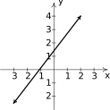
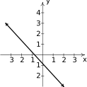
From the graphs above, we see that regardless if or , the range of linear functions is . Therefore, linear functions have no maximum or minimum.10
A couple of remarks about Example 1.2.3 are in order. First, if represents the number of PortaBoy game systems being produced, then can really only take on whole number values. We will revisit this scenario in Section 1.4 where we will see how the approach presented here allows us to use more elegant techniques when analyzing the situation than a discrete data set would allow.13
Second, once we know that the variable cost is per PortaBoy, we can revisit a computation we did earlier in the example. We computed and needed to compute . With being just one more PortaBoy than , we can use the variable cost to get
which agrees with our earlier computation.14 If we wanted to find , we could do something similar. Using , we can find as follows:
In general, we could rewrite . This same reasoning shows that for any in the domain of , we have - a fact we invite the reader to verify.15
Indeed, the computations above are at the heart of what it means to be a linear function: linear functions change at a constant rate known as the slope. To better see this algebraically, recall that given a point on a line along with the slope, , the point-slope form of the line is: .16 Rewriting, we get and setting and yields:
A few remarks are in order. First note that if the point is the -intercept , Equation 1.1 immediately reduces to the slope-intercept form of the line: so you can use Equation 1.1 exclusively from this point forward.17
Second, if we write , then so we can rewrite Equation 1.1 as follows:
In other words, changing the input by results in changing the output by . This tracks since
The fact that we can write for any choice of is another way to see that for linear functions, the rate of change is constant. That is, the rate of change, , is the same for all values in the domain. We'll put Equation 1.1 to good use in the next example.
The function in Example 1.2.4 is called the price-demand function (or, sometimes called more simply a `demand function') because it returns the price associated with a certain demand - that is, how many products will sell.21 These functions, along with cost functions like the one in Example 1.2.3, will be revisited in Example 1.4.3.
Our next two examples focus on writing formulas for piecewise-defined functions, the second of which models a real-world situation.
Linear Regression
We have demonstrated in this section that constant, linear, and piecewise combinations of these two function types can be used to model a variety of phenomena inspired by real-world situations. What happens, as if often the case in real-world situations, when we are given data sets that are not precisely linear, but still have a definite linear trend? An example of this is Skippy's time and temperature data from Example 1.1.1 in Section 1.1.
In that example, represented the time (number of hours after 6 a.m.) and represented the outdoor temperature in degrees Fahrenheit. The data Skippy collected along with a plot of the function are given below. Even though the data points as varies from to do not all lie on the same line - a fact we could prove analytically by checking slopes - there does appear to be a linear trend evident. The same can be said for the data as varies from to . As we'll see, there are statistical methods which can produce linear functions that are in some sense `closest' to all of the data, and they are represented below by the dashed lines below on the right.
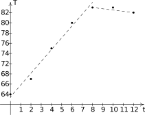
How do we measure how `close' a set of points is to a given line? Let's leave Skippy's data for the moment and focus on a smaller data set. Suppose we collected three data points: . At the top of the next page (on the left) we plot these points along with the line . The way we measure how close the line is to these points is by computing the total squared (vertical) error between the data points and the line as follows. For each of our data points, we find the vertical distance between the point and the line. To accomplish this, we need to find a point on the line directly above or below each data point. In other words, we need a point on the line with the same -coordinate as our data point.
For example, to find the point on the line directly above , we plug into and we get the point . Similarly, we find is on the line already and is the point on the line directly beneath . We find the total squared error by taking the sum of the squares of the differences of the -coordinates of each data point and its corresponding point on the line. For the data and line in this discussion .
Using advanced mathematical machinery,24 it is possible to find the line which results in the lowest value of . This line is called the least squares regression line, or sometimes the `line of best fit'. The formula for the line of best fit requires notation we won't present until Chapter 10, so we will revisit it then. Most graphing utilities have a built-in regression feature, so at this point we turn the computations over to the technology. A screenshot from desmos is given on the right at the top of the next page.
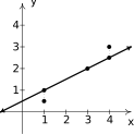
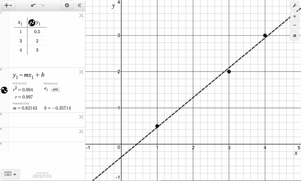
Our graphing utility produces the model25 where the slope is and the -coordinate of the -intercept is . The value is the correlation coefficient and is a measure of how close the data is to being on the same line. The closer is to , the better the linear fit.26 Having tells us that the points have a strong, positive correlation - that is, they are very close to being on a line with a positive slope, namely . Indeed, the total squared error between our data set and this line is . The mathematics tells us that this is the smallest we can get by modifying the parameters and , even though none of the data points actually lie on the line.
Now that we have this new mathematical machinery, let's revisit Skippy's time and temperature data.
Examples 1.2.3, 1.2.4 and 1.2.7 (among others) represent three different levels of mathematical modeling. In Example 1.2.3, the mathematical model (the cost function) was provided and our task was to use the model to interpret the mathematics in that context. In Example 1.2.4, we were given a minimal amount of information, namely, two data points, and then asked to construct a model which fit those data exactly. Lastly, in Example 1.2.7, we were given several data points and we used statistical methods to construct a best fit model to the data.
The validity of the models rests on the validity of the underlying assumptions used to create the models. For instance, is there any reason to assume a price-demand function would be linear? Is it reasonable to assume that the temperature changes at a constant rate? These are questions for economists and scientists. Mathematicians often take on a role of equal parts translator and prophet: they codify ideas into formulas and then use them to make predictions about yet-to-be observed phenomena.
The Average Rate of Change of a Function
As mentioned earlier in the section, the concepts of slope and the more general rates of change are important concepts not just in Mathematics, but also in other fields. Many important phenomena are modeled using non-linear functions, and while the rates of change of these functions are not constant, we can sample the function at two points and compute what is known as an average rate of change between them to give some sense as to the function's behavior over that interval.29
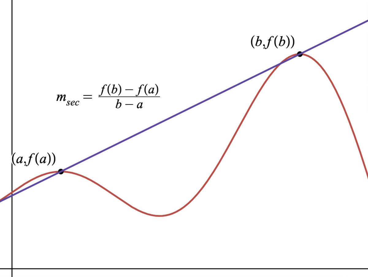
The graph of a function along with the secant line through the points and .
As with Definitions 1.3 and 1.7, the wording in Definition 1.8, while referring to the function , is really making a statement about its outputs .
If is increasing over , then the average rate of change will be positive. Likewise, if is decreasing or constant, the average rate of change will be negative or , respectively. (Think about this for a moment.) However, as the next example demonstrates, the converses of these statements aren't always true.31
An important lesson from the last example is that average rates of change give us a snapshot of what is happening at the endpoints of an interval, but not necessarily what happens over the course of the interval. Calculus gives us tools to compute slopes at points which correspond to instantaneous rates of changes. While we don't quite have the machinery to properly express these ideas, we can hint at them in the Exercises. Speaking of exercises …
Exercises
In Exercises -, graph the function. Find the slope and axis intercepts, if any.
In Exercises -, graph the function. Find the domain, range, and axis intercepts, if any.
The unit step function is defined as
- Graph .
- State the domain and range of .
- List the interval(s) over which is increasing, decreasing, and/or constant.
- Write as a piecewise defined function and graph.
In Exercises -, find a formula for the function.
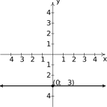
Figure 1.81 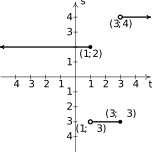
Figure 1.82 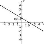
Figure 1.83 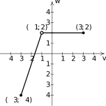
Figure 1.84 For copies of the book Me and my Sasquatch, a print on-demand company charges dollars, where is determined by the formula
- Find and interpret .
- How much does it cost to order 50 copies of the book? What about 51 copies?
- Your answer to should get you thinking. Suppose a bookstore estimates it will sell 50 copies of the book. How many books can, in fact, be ordered for the same price as those 50 copies? (Round your answer to a whole number of books.)
An on-line comic book retailer charges shipping costs according to the following formula
where is the number of comic books purchased and is the shipping cost in dollars.
- What is the cost to ship 10 comic books?
- What is the significance of the formula for ?
The cost in dollars to talk minutes a month on a mobile phone plan is modeled by
- How much does it cost to talk minutes per month with this plan?
- How much does it cost to talk hours a month with this plan?
- Explain the terms of the plan verbally.
- Jeff can walk comfortably at miles per hour. Find an expression for a linear function that represents the total distance Jeff can walk in hours, assuming he doesn't take any breaks.
- Carl can stuff envelopes per minute. Find an expression for a linear function that represents the total number of envelopes Carl can stuff after hours, assuming he doesn't take any breaks.
- A landscaping company charges per cubic yard of mulch plus a delivery charge of . Find an expression for a linear function which computes the total cost in dollars to deliver cubic yards of mulch.
- A plumber charges for a service call plus per hour. If she spends no longer than 8 hours a day at any one site, find an expression for a linear function that computes her total daily charges in dollars as a function of the amount of time spent in hours, at any one given location.
- A salesperson is paid $200 per week plus 5% commission on her weekly sales of dollars. Find an expression for a linear function which computes her total weekly pay in dollars as a function of . What must her weekly sales be in order for her to earn $475.00 for the week?
- An on-demand publisher charges to print a 600 page book and to print a 400 page book. Find an expression for a linear function which models the cost of a book in dollars as a function of the number of pages . Find and interpret both the slope of the linear function and .
- The Topology Taxi Company charges for the first fifth of a mile and for each additional fifth of a mile. Find an expression for a linear function which models the taxi fare as a function of the number of miles driven, . Find and interpret both the slope of the linear function and .
Water freezes at Celsius and Fahrenheit and it boils at C and F.
- Find an expression for a linear function that computes temperature in the Fahrenheit scale as a function of the temperature given in degrees Celsius. Use this function to convert C into Fahrenheit.
- Find an expression for a linear function that computes temperature in the Celsius scale as a function of the temperature given in degrees Fahrenheit. Use this function to convert F into Celsius.
- Is there a temperature such that ?
- Legend has it that a bull Sasquatch in rut will howl approximately 9 times per hour when it is outside and only 5 times per hour if it's . Assuming that the number of howls per hour, , can be represented by a linear function of temperature Fahrenheit, find the number of howls per hour he'll make when it's only outside. What troubles do you encounter when trying to determine a reasonable applied domain?
- Economic forces have changed the cost function for PortaBoys to . Rework Example 1.2.3 with this new cost function.
- In response to the economic forces in Exercise above, the local retailer sets the selling price of a PortaBoy at $250. Remarkably, 30 units were sold each week. When the systems went on sale for $220, 40 units per week were sold. Rework Example 1.2.4 with this new data.
- A local pizza store offers medium two-topping pizzas delivered for per pizza plus a delivery charge per order. On weekends, the store runs a `game day' special: if six or more medium two-topping pizzas are ordered, they are each with no delivery charge. Write a piecewise-defined linear function which calculates the cost in dollars of medium two-topping pizzas delivered during a weekend.
- A restaurant offers a buffet which costs per person. For parties of or more people, a group discount applies, and the cost is per person. Write a piecewise-defined linear function which calculates the total bill of a party of people who all choose the buffet.
A mobile plan charges a base monthly rate of for the first minutes of air time plus a charge of ¢ for each additional minute. Write a piecewise-defined linear function which calculates the monthly cost in dollars for using minutes of air time.
HINT: You may wish to refer to number for inspiration.
- The local pet shop charges ¢ per cricket up to 100 crickets, and ¢ per cricket thereafter. Write a piecewise-defined linear function which calculates the price in dollars of purchasing crickets.
The cross-section of a swimming pool is below. Write a piecewise-defined linear function which describes the depth of the pool, (in feet) as a function of:
- the distance (in feet) from the edge of the shallow end of the pool, .
- the distance (in feet) from the edge of the deep end of the pool, .
- Graph each of the functions in (a) and (b). Discuss with your classmates how to transform one into the other and how they relate to the diagram of the pool.
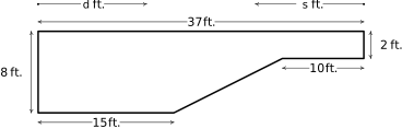
Figure 1.85 - The function defined by is called the Identity Function. Thinking from a procedural perspective, explain a possible origin of this name.
Why must the graph of a function have at most one -intercept?
HINT: Consider what would happen graphically if there were more than one …
- Why is a discussion of vertical lines omitted when discussing functions?
- Find a formula for the -intercept of the graph of . Assume .
- Suppose is the -intercept of a linear function . Use the point-slope form of a liner function, Equation 1.1 to show . This is the `slope -intercept' form of the linear function.
- Prove that for all linear functions with with slope , .
Find the slopes between the following points from the data set given in Example 1.2.7 and compare them with the slope of the corresponding regression line:
- ,
- ,
- ,
- ,
According to this website 32, the census data for Lake County, Ohio is:
Table 1.1 Year 1970 1980 1990 2000 Population 197200 212801 215499 227511 - Find the least squares regression line for these data and comment on the goodness of fit.33 Interpret the slope of the line of best fit.
- Use the regression line to predict the population of Lake County in 2010. (The recorded figure from the 2010 census is )
- Use the regression line to predict when the population of Lake County will reach .
According to this website 34, the census data for Lorain County, Ohio is:
Table 1.2 Year 1970 1980 1990 2000 Population 256843 274909 271126 284664 - Find the least squares regression line for these data and comment on the goodness of fit. Interpret the slope of the line of best fit.
- Use the regression line to predict the population of Lorain County in 2010. (The recorded figure from the 2010 census is )
- Use the regression line to predict when the population of Lake County will reach .
The chart below contains a portion of the fuel consumption information for a 2002 Toyota Echo that Jeffrey used to own. The first row is the cumulative number of gallons of gasoline that I had used and the second row is the odometer reading when I refilled the gas tank. So, for example, the fourth entry is the point (28.25, 1051) which says that I had used a total of 28.25 gallons of gasoline when the odometer read 1051 miles.
Table 1.3 Gasoline Used (Gallons) 0 9.26 19.03 28.25 36.45 44.64 53.57 62.62 71.93 81.69 90.43 Odometer (Miles) 41 356 731 1051 1347 1631 1966 2310 2670 3030 3371 Find the least squares line for this data. Is it a good fit? What does the slope of the line represent? Do you and your classmates believe this model would have held for ten years had I not crashed the car on the Turnpike a few years ago?
Using the energy production data given below
Table 1.4 Year 1950 1960 1970 1980 1990 2000 Production (in Quads) 35.6 42.8 63.5 67.2 70.7 71.2 - Plot the data using a graphing utility and explain why it does not appear to be linear.
- Discuss with your classmates why ignoring the first two data points may be justified from a historical perspective.
- Find the least squares regression line for the last four data points and comment on the goodness of fit. Interpret the slope of the line of best fit.
- Use the regression line to predict the annual US energy production in the year .
- Use the regression line to predict when the annual US energy production will reach Quads.
In Exercises -, compute the average rate of change of the function over the specified interval.
- The height of an object dropped from the roof of a building is modeled by: , for . Here, is the height of the object off the ground in feet seconds after the object is dropped. Find and interpret the average rate of change of over the interval .
- Using data from Bureau of Transportation Statistics , the average fuel economy in miles per gallon for passenger cars in the US can be modeled by , , where is the number of years since . Find and interpret the average rate of change of over the interval .
The temperature in degrees Fahrenheit hours after 6 AM is given by:
- Find and interpret , and .
- Find and interpret the average rate of change of over the interval .
- Find and interpret the average rate of change of from to .
- Find and interpret the average rate of temperature change between 10 AM and 6 PM.
- Suppose represents the costs, in hundreds, to produce thousand pens. Find and interpret the average rate of change as production is increased from making 3000 to 5000 pens.
Recall from Example 1.2.8 The formula for gives the height, , measured in feet, of a model rocket above the Moon's surface as a function of the time after lift-off, , in seconds.
Find and interpret the average rate of change of over the following intervals:
- What value does the average rate of change appear to be approaching as the interval shrinks closer to the value ?
- Find the equation of the line containing with slope and graph it along with on the same set of axes using a graphing utility. What happens as you zoom in near ?
- Show the average rate of change of a function of the form over any interval is .
- Why doesn't the graph of the vertical line in the -plane represent as a function of ?
With help from a graphing utility, graph the following pairs of functions on the same set of axes:35
- and
- and
- and
- and
Choose more functions and graph alongside until you can explain how, in general, one would obtain the graph of given the graph of .
The Lagrange Interpolate function for two points and where is given by:
For each of the following pairs of points, find using the formula above and verify each of the points lies on the graph of .
- ,
- ,
- ,
- ,
- Verify that, in general, and .
- Show the point-slope form of a linear function, Equation 1.1 is equivalent to the formula given for after making the identifications: and .
Answers
slope:
-intercept:
-intercept:
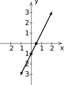
Figure 1.86 slope:
-intercept:
-intercept:
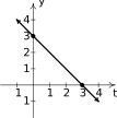
Figure 1.87 slope:
-intercept:
-intercept: none

Figure 1.88 slope:
-intercept:
-intercept:

Figure 1.89 slope:
-intercept:
-intercept:

Figure 1.90 slope:
-intercept:
-intercept:

Figure 1.91 domain:
range:
-intercept:
-intercept: none
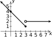
Figure 1.92 domain:
range:
-intercept:
-intercept:
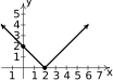
Figure 1.93 domain:
range:
-intercept:
-intercepts: ,
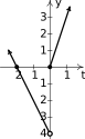
Figure 1.94 domain:
range:
-intercept:
-intercept:
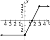
Figure 1.95 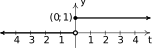
Figure 1.96 - domain: , range:
- is constant on and .
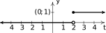
Figure 1.97
- . It costs for 20 copies of the book.
- , . , .
- 56 books.
- , .
- There is free shipping on orders of or more comic books.
- , .
- , .
- It costs for up to minutes and cents per minute for each minute over minutes.
- , .
- , .
- , .
- , .
- She must make $5500 in weekly sales.
- The slope means it costs ¢ per page. means there is a fixed, or start-up, cost of to make each book.
- The slope means it costs an additional for each mile beyond the first 0.2 miles. , so according to the model, it would cost for a trip of miles. Would this ever really happen? Depends on the driver and the passenger, we suppose.
- .
and howls per hour.
Having a negative number of howls makes no sense and since we can put an upper bound of on the domain. The lower bound is trickier because there's nothing other than common sense to go on. As it gets colder, he howls more often. At some point it will either be so cold that he freezes to death or he's howling non-stop. So we're going to say that he can withstand temperatures no lower than so that the applied domain is .
, so our start-up costs are . , so to produce systems, it costs .
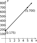
Figure 1.98 - Since we can't make a negative number of game systems, .
- The slope is so for each additional system produced, it costs an additional .
- Solving gives so can be produced for .
, .
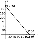
Figure 1.99 - The slope is so for each drop in price, we sell one additional game system.
- Since is not in the domain of , is not defined. (In other words, under these conditions, it is impossible to sell 150 game systems.)
- Solving gives so if the price per system, we would sell systems.
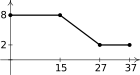
Figure 1.100 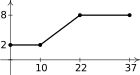
Figure 1.101
- Since for all real numbers , the function doesn't change the `identity' of the input at all.
- If a graph contains more than one -intercept, it would violate the Vertical Line Test since would be matched with (at least) two different -values.
- Vertical Lines fail the Vertical Line Test.
- . (Note the importance here of .)
- Plugging in for , we get or .
- Since is linear with slope , .
The first two points contributed to a regression line slope of ; the last two points contributed to a regression line slope of .
- with which indicates a good fit. The slope indicates Lake County's population is increasing at a rate of (approximately) 936 people per year.
- According to the model, the population in 2010 will be .
- According to the model, the population of Lake County will reach sometime between 2024 and 2025.
- with which indicates a reasonable fit. The slope indicates Lorain County's population is increasing at a rate of (approximately) 797 people per year.
- According to the model, the population in 2010 will be .
- According to the model, the population of Lake County will reach sometime between 2051 and 2052.
- The regression line is with , so this is an excellent fit. The slope represents mileage in miles per gallon.
- with which indicates a good fit. The slope indicates the country's energy production is increasing at a rate of Quad per year.
- According to the model, the production in 2010 will be Quad.
- According to the model, the production will reach Quad in the year 2105.
- The average rate of change is . During the first two seconds after it is dropped, the object has fallen at an average rate of feet per second.
- The average rate of change is . From 1980 to 2008, the average fuel economy of passenger cars in the US increased, on average, at a rate of miles per gallon per year.
- , so at 10 AM (4 hours after 6 AM), it is F. , so at 2 PM (8 hours after 6 AM), it is F. , so at 6 PM (12 hours after 6 AM), it is F.
- The average rate of change is . Between 10 AM and 2 PM, the temperature increases, on average, at a rate of F per hour.
- The average rate of change is . Between 2 PM and 6 PM, the temperature decreases, on average, at a rate of F per hour.
- The average rate of change is . Between 10 AM and 6 PM, the temperature, on average, remains constant.
- The average rate of change is . As production is increased from 3000 to 5000 pens, the cost decreases at an average rate of per 1000 pens produced (20¢ per pen.)
- so the average velocity of the rocket between and seconds after lift off is feet per second ( feet per second directed downwards.)
- so the average velocity of the rocket between and seconds after lift off is feet per second. ( feet per second directed downwards.)
- so the average velocity of the rocket between and seconds after lift off is feet per second. ( feet per second directed downwards.)
- so the average velocity of the rocket between and seconds after lift off is feet per second. ( feet per second directed downwards.)
- The average rate of change seem to be approaching .
- Line: or . Graphing this line along with the on a graphing utility we find the two graphs become indistinguishable as we zoom in near .
Adapted from Precalculus with Integrated Calculus, edition 4i, by Carl Stitz and Jeff Zeager (stitz-zeager.com), licensed under CC BY-NC-SA 3.0. Changes were made: reformatted as an accessible XYZ web edition. License: CC-BY-NC-SA-3.0.