In the previous section, we introduced sequences and now we shall present notation and theorems concerning the sum of terms of a sequence. We begin with a definition, which, while intimidating, is meant to make our lives easier.
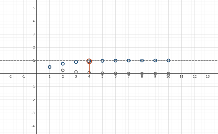
Interactive figureSummation as a running total: the partial sums S_n climb toward the limitDrag the Upper limit n slider from 1 to 10.
XYZ Graph · viewer build 5edf91b
The gray dots are the terms a_k = 1/2^k, halving at every step. The navy dots are the partial sums S_n = a₁ + … + a_n, which the summation notation Σ abbreviates; each navy dot sits exactly the next gray term's height above the previous one, and the closed form S_n = 1 − 1/2^n says why the dots approach the dashed line y = 1 without reaching it. Slide the upper limit n and the rust marker shows which running total the symbol Σ_{k=1}^{n} a_k names.
In English, Definition 9.3 is simply defining a short-hand notation for adding up the terms of the sequence from through . The symbol is the capital Greek letter sigma and is shorthand for `sum'. The lower and upper limits of the summation tells us which term to start with and which term to end with, respectively. For example, using the sequence for , we can write the sum as
The index variable is considered a `dummy variable' in the sense that it may be changed to any letter without affecting the value of the summation. For instance,
One place you may encounter summation notation is in mathematical definitions. For example, summation notation allows us to define polynomials as functions of the form
for real numbers , . The reader is invited to compare this with what is given in Definition 3.1. Summation notation is particularly useful when talking about matrix operations. For example, we can write the product of the th row of a matrix and the column of a matrix as
Again, the reader is encouraged to write out the sum and compare it to Definition 8.9. Our next example gives us practice with this new notation.
The following theorem presents some general properties of summation notation. While we shall not have much need of these properties in Algebra, they do play a great role in Calculus. Moreover, there is much to be learned by thinking about why the properties hold. We invite the reader to prove these results. To get started, remember, “When in doubt, write it out!”
We now turn our attention to the sums involving arithmetic and geometric sequences. Given an arithmetic sequence for , we let denote the sum of the first terms. To derive a formula for , we write it out in two different ways
If we add these two equations and combine the terms which are aligned vertically, we get
The right hand side of this equation contains terms, all of which are equal to so we get . Dividing both sides of this equation by , we obtain the formula
If we rewrite the quantity as , we get the formula
A helpful way to remember this last formula is to recognize that we have expressed the sum as the product of the number of terms and the average of the first and terms.
To derive the formula for the geometric sum, we start with a geometric sequence , , and let once again denote the sum of the first terms. Comparing and , we get
Subtracting the second equation from the first forces all of the terms except and to cancel out and we get . Factoring, we get . Assuming , we can divide both sides by the quantity to obtain
If we distribute through the numerator, we get which yields the formula
In the case when , we get the formula
Our results are summarized below.
While we have made an honest effort to derive the formulas in Equation 9.2, formal proofs require the machinery in Section 9.3. An application of the arithmetic sum formula which proves useful in Calculus results in formula for the sum of the first natural numbers. The natural numbers themselves are a sequence4
, , , …which is arithmetic with . Applying Equation 9.2,
So, for example, the sum of the first natural numbers5 is .
An important application of the geometric sum formula is the investment plan called an annuity. Annuities differ from the kind of investments we studied in Section 6.5 in that payments are deposited into the account on an on-going basis, and this complicates the mathematics a little.6 Suppose you have an account with annual interest rate which is compounded times per year. We let denote the interest rate per period. Suppose we wish to make ongoing deposits of dollars at the end of each compounding period. Let denote the amount in the account after compounding periods. Then , because we have made our first deposit at the end of the first compounding period and no interest has been earned. During the second compounding period, we earn interest on so that our initial investment has grown to in accordance with Equation 6.1. When we add our second payment at the end of the second period, we get
The reason for factoring out the will become apparent in short order. During the third compounding period, we earn interest on which then grows to . We add our third payment at the end of the third compounding period to obtain
During the fourth compounding period, grows to , and when we add the fourth payment, we factor out to get
This pattern continues so that at the end of the th compounding, we get
The sum in the parentheses above is the sum of the first terms of a geometric sequence with and . Using Equation 9.2, we get
Hence, we get
If we let be the number of years this investment strategy is followed, then , and we get the formula for the future value of an ordinary annuity.
The reader is encouraged to substitute into Equation 9.3 and simplify. Some familiar equations arise which are cause for pause and meditation. One last note: if the deposit is made a the beginning of the compounding period instead of at the end, the annuity is called an annuity-due. We leave the derivation of the formula for the future value of an annuity-due as an exercise for the reader.
We close this section with a peek into Calculus by considering infinite sums, called series. Consider the number . We can write this number as
From Example 9.2.1, we know we can write the sum of the first of these terms as
Using Equation 9.2, we have
It stands to reason that is the same value of as . Our knowledge of exponential expressions from Section 6.1 tells us that as , so . We have just argued that , which may cause some distress for some readers.7 Any non-terminating decimal can be thought of as an infinite sum whose denominators are the powers of , so the phenomenon of adding up infinitely many terms and arriving at a finite number is not as foreign of a concept as it may appear. We end this section with a theorem concerning geometric series.
The justification of the result in Theorem 9.2 comes from taking the formula in Equation 9.2 for the sum of the first terms of a geometric sequence and examining the formula as . Assuming means , so as . Hence as ,
As to what goes wrong when , we leave that to Calculus as well, but will explore some cases in the exercises.
Exercises
In Exercises -, find the value of each sum using Definition 9.3.
In Exercises -, rewrite the sum using summation notation.
In Exercises -, use the formulas in Equation 9.2 to find the sum.
In Exercises -, use Theorem 9.2 to express each repeating decimal as a fraction of integers.
In Exercises -, use Equation 9.3 to compute the future value of the annuity with the given terms. In all cases, assume the payment is made monthly, the interest rate given is the annual rate, and interest is compounded monthly.
payments are $300, interest rate is 2.5%, term is 17 years.
payments are $50, interest rate is 1.0%, term is 30 years.
payments are $100, interest rate is 2.0%, term is 20 years
payments are $100, interest rate is 2.0%, term is 25 years
payments are $100, interest rate is 2.0%, term is 30 years
payments are $100, interest rate is 2.0%, term is 35 years
Suppose an ordinary annuity offers an annual interest rate of , compounded monthly, for 30 years. What should the monthly payment be to have at the end of the term?
Prove the properties listed in Theorem 9.1.
Show that the formula for the future value of an annuity due is
Discuss with your classmates what goes wrong when trying to find the following sums.8
Answers
$76,163.67
For , the monthly payment is .
Adapted from Precalculus, 3rd corrected edition, by Carl Stitz and Jeff Zeager (stitz-zeager.com), licensed under CC BY-NC-SA 3.0. Changes were made: reformatted as an accessible XYZ web edition. License: CC-BY-NC-SA-3.0.
These eBooks are a prerelease and are not yet certified conformant with WCAG 2.1 AA or ADA Title II. Every page is built against an automated accessibility gate, and the published editions will meet ADA Title II requirements when they release in late September 2026. If something is unusable, please tell us.