In this section we will develop techniques for solving equations involving exponential functions. Suppose, for instance, we wanted to solve the equation . After a moment's calculation, we find , so we have . The one-to-one property of exponential functions, detailed in Theorem 6.4, tells us that if and only if . This means that not only is a solution to , it is the only solution. Now suppose we change the problem ever so slightly to . We could use one of the inverse properties of exponentials and logarithms listed in Theorem 6.3 to write . We'd then have , which means our solution is . This makes sense because, after all, the definition of is `the exponent we put on to get .' Indeed we could have obtained this solution directly by rewriting the equation in its logarithmic form . Either way, in order to get a reasonable decimal approximation to this number, we'd use the change of base formula, Theorem 6.7, to give us something more calculator friendly,1 say . Another way to arrive at this answer is as follows
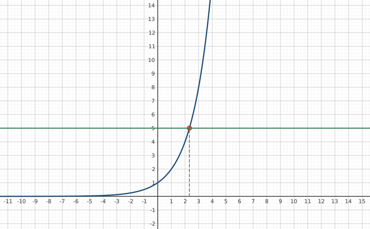
Interactive figureSolving a^x = c by sight: the crossing sits at x = log_a(c)Drag the Base a and Line height c sliders.
XYZ Graph · viewer build 5edf91b
The equation a^x = c asks where the exponential curve y = a^x crosses the horizontal line y = c. The marked crossing is the solution, and its x-coordinate is exactly log_a(c) = ln(c)/ln(a), which the dashed drop to the x-axis reads off. Slide the base a and the line height c: a larger base reaches the line sooner, a higher line pushes the crossing to the right, and a line at or below zero never meets the curve at all, which is the graphical face of the domain of the logarithm.
`Taking the natural log' of both sides is akin to squaring both sides: since is a function, as long as two quantities are equal, their natural logs are equal.2 Also note that we treat as any other non-zero real number and divide it through3 to isolate the variable . We summarize below the two common ways to solve exponential equations, motivated by our examples.
Steps for Solving an Equation involving Exponential Functions
Isolate the exponential function.
If convenient, express both sides with a common base and equate the exponents.
Otherwise, take the natural log of both sides of the equation and use the Power Rule.
The authors would be remiss not to mention that Example 6.3.1 still holds great educational value. Much can be learned about logarithms and exponentials by verifying the solutions obtained in Example 6.3.1 analytically. For example, to verify our solution to , we substitute and obtain
The other solutions can be verified by using a combination of log and inverse properties. Some fall out quite quickly, while others are more involved. We leave them to the reader.
Since exponential functions are continuous on their domains, the Intermediate Value Theorem 3.1 applies. As with the algebraic functions in Section 5.3, this allows us to solve inequalities using sign diagrams as demonstrated below.
We close this section by finding the inverse of a function which is a composition of a rational function with an exponential function.
Exercises
In Exercises -, solve the equation analytically.
In Exercises -, solve the inequality analytically.
In Exercises -, use your calculator to help you solve the equation or inequality.
Since is a strictly increasing function, if then . Use this fact to solve the inequality without a sign diagram. Use this technique to solve the inequalities in Exercises -. (NOTE: Isolate the exponential function first!)
Compute the inverse of . State the domain and range of both and .
In Example 6.3.4, we found that the inverse of was but we left a few loose ends for you to tie up.
Show that for all in the domain of and that for all in the domain of .
Find the range of by finding the domain of .
Let and . Show that and that . (We know this is true in general by Exercise in Section 5.2, but it's nice to see a specific example of the property.)
With the help of your classmates, solve the inequality for a variety of natural numbers . What might you conjecture about the “speed” at which grows versus any polynomial?
Answers
No solution.
,
. Both and have domain and range .
Adapted from Precalculus, 3rd corrected edition, by Carl Stitz and Jeff Zeager (stitz-zeager.com), licensed under CC BY-NC-SA 3.0. Changes were made: reformatted as an accessible XYZ web edition. License: CC-BY-NC-SA-3.0.
These eBooks are a prerelease and are not yet certified conformant with WCAG 2.1 AA or ADA Title II. Every page is built against an automated accessibility gate, and the published editions will meet ADA Title II requirements when they release in late September 2026. If something is unusable, please tell us.