
5.3 Other Algebraic Functions
This section serves as a watershed for functions which are combinations of polynomial, and more generally, rational functions, with the operations of radicals. It is business of Calculus to discuss these functions in all the detail they demand so our aim in this section is to help shore up the requisite skills needed so that the reader can answer Calculus's call when the time comes. We briefly recall the definition and some of the basic properties of radicals from Intermediate Algebra.1
It is worth remarking that, in light of Section 5.2, we could define functionally as the inverse of with the stipulation that when is even, the domain of is restricted to . From what we know about from Section 3.1 along with Theorem 5.3, we can produce the graphs of by reflecting the graphs of across the line . Below are the graphs of , and . The point is indicated as a reference. The axes are hidden so we can see the vertical steepening near and the horizontal flattening as .


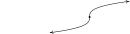
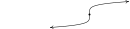
The odd-indexed radical functions also follow a predictable trend - steepening near and flattening as . In the exercises, you'll have a chance to graph some basic radical functions using the techniques presented in Section 1.7.

We have used all of the following properties at some point in the textbook for the case (the square root), but we list them here in generality for completeness.
The proof of Theorem 5.6 is based on the definition of the principal roots and properties of exponents. To establish the product rule, consider the following. If is odd, then by definition is the unique real number such that . Given that , it must be the case that . If is even, then is the unique non-negative real number such that . Also note that since is even, and are also non-negative and hence so is . Proceeding as above, we find that . The quotient rule is proved similarly and is left as an exercise. The power rule results from repeated application of the product rule, so long as is a real number to start with.4 The last property is an application of the power rule when is odd, and the occurrence of the absolute value when is even is due to the requirement that in Definition 5.4. For instance, , not . It's this last property which makes compositions of roots and powers delicate. This is especially true when we use exponential notation for radicals. Recall the following definition.
The rational exponents defined in Definition 5.5 behave very similarly to the usual integer exponents from Elementary Algebra with one critical exception. Consider the expression . Applying the usual laws of exponents, we'd be tempted to simplify this as . However, if we substitute and apply Definition 5.5, we find so that . We see in this case that . If we take the time to rewrite with radicals, we see
In the play-by-play analysis, we see that when we canceled the 's in multiplying , we were, in fact, attempting to cancel a square with a square root. The fact that and not simply is the root6 of the trouble. It may amuse the reader to know that , and this verification is left as an exercise. The moral of the story is that when simplifying fractional exponents, it's usually best to rewrite them as radicals.7 The last major property we will state, and leave to Calculus to prove, is that radical functions are continuous on their domains, so the Intermediate Value Theorem, Theorem 3.1, applies. This means that if we take combinations of radical functions with polynomial and rational functions to form what the authors consider the algebraic functions,8 we can make sign diagrams using the procedure set forth in Section 4.2.
Steps for Constructing a Sign Diagram for an Algebraic Function
Suppose is an algebraic function.
- Place any values excluded from the domain of on the number line with an `‽' above them.
- Find the zeros of and place them on the number line with the number above them.
- Choose a test value in each of the intervals determined in steps 1 and 2.
- Determine the sign of for each test value in step 3, and write that sign above the corresponding interval.
Our next example reviews quite a bit of Intermediate Algebra and demonstrates some of the new features of these graphs.
As the previous example illustrates, the graphs of general algebraic functions can have features we've seen before, like vertical and horizontal asymptotes, but they can occur in new and exciting ways. For example, had two distinct horizontal asymptotes. You'll recall that rational functions could have at most one horizontal asymptote. Also some new characteristics like `unusual steepness'11 and cusps12 can appear in the graphs of arbitrary algebraic functions. Our next example first demonstrates how we can use sign diagrams to solve nonlinear inequalities. (Don't panic. The technique is very similar to the ones used in Chapters 2, 3 and 4.) We then check our answers graphically with a calculator and see some of the new graphical features of the functions in this extended family.
One application of algebraic functions was given in Example 1.6.6 in Section 1.1. Our last example is a more sophisticated application of distance.
Exercises
For each function in Exercises - below
- Find its domain.
- Create a sign diagram.
- Use your calculator to help you sketch its graph and identify any vertical or horizontal asymptotes, `unusual steepness' or cusps.
In Exercises -, sketch the graph of by starting with the graph of and using the transformations presented in Section 1.7.
- ,
- ,
- ,
- ,
- ,
- ,
In Exercises -, solve the equation or inequality.
- Rework Example 5.3.3 so that the outpost is 10 miles from Route 117 and the nearest junction box is 30 miles down the road for the post.
The volume of a right cylindrical cone depends on the radius of its base and its height and is given by the formula . The surface area of a right cylindrical cone also depends on and according to the formula . Suppose a cone is to have a volume of 100 cubic centimeters.
- Use the formula for volume to find the height as a function of .
- Use the formula for surface area and your answer to to find the surface area as a function of .
- Use your calculator to find the values of and which minimize the surface area. What is the minimum surface area? Round your answers to two decimal places.
The National Weather Service uses the following formula to calculate the wind chill:
where is the wind chill temperature in F, is the air temperature in F, and is the wind speed in miles per hour. Note that is defined only for air temperatures at or lower than F and wind speeds above miles per hour.
- Suppose the air temperature is and the wind speed is miles per hour. Find the wind chill temperature. Round your answer to two decimal places.
- Suppose the air temperature is F and the wind chill temperature is F. Find the wind speed. Round your answer to two decimal places.
As a follow-up to Exercise, suppose the air temperature is F.
- Use the formula from Exercise to find an expression for the wind chill temperature as a function of the wind speed, .
- Solve , round your answer to two decimal places, and interpret.
- Graph the function using your calculator and check your answer to part.
The period of a pendulum in seconds is given by
(for small displacements) where is the length of the pendulum in meters and meters per second per second is the acceleration due to gravity. My Seth-Thomas antique schoolhouse clock needs second and I can adjust the length of the pendulum via a small dial on the bottom of the bob. At what length should I set the pendulum?
The Cobb-Douglas production model states that the yearly total dollar value of the production output in an economy is a function of labor (the total number of hours worked in a year) and capital (the total dollar value of all of the stuff purchased in order to make things). Specifically, . By fixing , we create what's known as an `isoquant' and we can then solve for as a function of . Let's assume that the Cobb-Douglas production model for the country of Sasquatchia is .
- Let and solve for in terms of . If , what is ?
- Graph the isoquant . What information does an ordered pair which makes give you? With the help of your classmates, find several different combinations of labor and capital all of which yield . Discuss any patterns you may see.
According to Einstein's Theory of Special Relativity, the observed mass of an object is a function of how fast the object is traveling. Specifically,
where is the mass of the object at rest, is the speed of the object and is the speed of light.
- Find the applied domain of the function.
- Compute and .
- As , what happens to ?
- How slowly must the object be traveling so that the observed mass is no greater than 100 times its mass at rest?
- Find the inverse of .
Suppose Fritzy the Fox, positioned at a point in the first quadrant, spots Chewbacca the Bunny at . Chewbacca begins to run along a fence (the positive -axis) towards his warren. Fritzy, of course, takes chase and constantly adjusts his direction so that he is always running directly at Chewbacca. If Chewbacca's speed is and Fritzy's speed is , the path Fritzy will take to intercept Chewbacca, provided is directly proportional to, but not equal to, is modeled by
- Determine the path that Fritzy will take if he runs exactly twice as fast as Chewbacca; that is, . Use your calculator to graph this path for . What is the significance of the -intercept of the graph?
- Determine the path Fritzy will take if Chewbacca runs exactly twice as fast as he does; that is, . Use your calculator to graph this path for . Describe the behavior of as and interpret this physically.
- With the help of your classmates, generalize parts (a) and (b) to two cases: and . We will discuss the case of in Exercise in Section 6.5.
- Verify the Quotient Rule for Radicals in Theorem 5.6.
- Show that for all .
- Show that is an irrational number by first showing that it is a zero of and then showing has no rational zeros. (You'll need the Rational Zeros Theorem, Theorem 3.9, in order to show this last part.)
- With the help of your classmates, generalize Exercise to show that is an irrational number for any natural numbers and provided that for some natural number .
Answers
Domain:

Figure 5.48 No asymptotes Unusual steepness at and No cusps
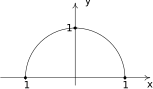
Figure 5.49 Domain:
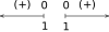
Figure 5.50 No asymptotes Unusual steepness at and No cusps
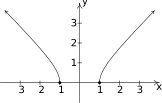
Figure 5.51 Domain:
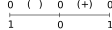
Figure 5.52 No asymptotes Unusual steepness at and No cusps
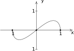
Figure 5.53 Domain:
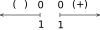
Figure 5.54 No asymptotes Unusual steepness at and No cusps
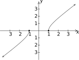
Figure 5.55 Domain:
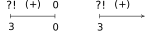
Figure 5.56 Vertical asymptotes: and Horizontal asymptote: Unusual steepness at No cusps
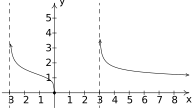
Figure 5.57 Domain:
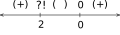
Figure 5.58 Vertical asymptote Horizontal asymptote No unusual steepness or cusps
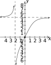
Figure 5.59 Domain:
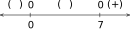
Figure 5.60 No vertical or horizontal asymptotes16 Unusual steepness at Cusp at
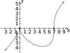
Figure 5.61 Domain:

Figure 5.62 No asymptotes Unusual steepness at No cusps
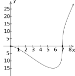
Figure 5.63 Domain:
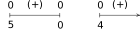
Figure 5.64 No asymptotes Unusual steepness at and No cusps
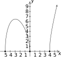
Figure 5.65 Domain:
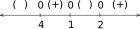
Figure 5.66 No vertical or horizontal asymptotes17 Unusual steepness at and No cusps
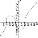
Figure 5.67 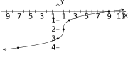
Figure 5.68 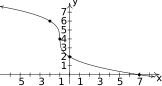
Figure 5.69 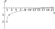
Figure 5.70 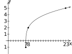
Figure 5.71 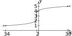
Figure 5.72 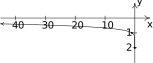
Figure 5.73 - , . The calculator gives the absolute minimum at . This means to minimize the cost, approximately 18.66 miles of cable should be run along Route 117 before turning off the road and heading towards the outpost. The minimum cost to run the cable is approximately .
- , .
- ,
- The calculator gives the absolute minimum at the point . This means the radius should be (approximately) 4.07 centimeters and the height should be 5.76 centimeters to give a minimum surface area of 90.23 square centimeters.
- F.
- miles per hour.
- . Since we are told in Exercise that wind chill is only effect for wind speeds of more than 3 miles per hour, we restrict the domain to .
- when . This means, according to the model, for the wind chill temperature to be F, the wind speed needs to be miles per hour.
The graph is below.
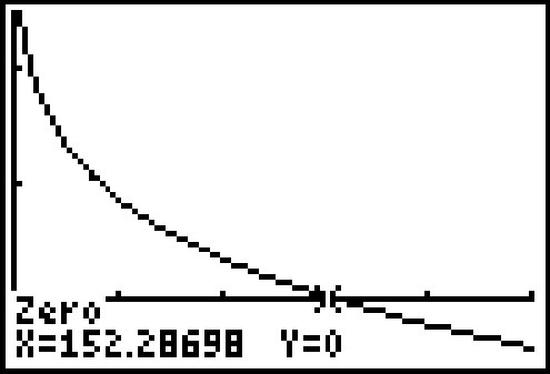
Figure 5.74
- meters or centimeters
- First rewrite the model as . Then yields . If then .
Table 5.13 - As
- If the object is traveling no faster than approximately times the speed of light, then its observed mass will be no greater than .
- . The point is when Fritzy's path crosses Chewbacca's path - in other words, where Fritzy catches Chewbacca.
. Using the techniques from Chapter 4, we find as , which means, in this case, Fritzy's pursuit never ends; he never catches Chewbacca. This makes sense since Chewbacca has a head start and is running faster than Fritzy.
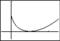
Figure 5.75 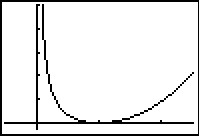
Figure 5.76
Adapted from Precalculus, 3rd corrected edition, by Carl Stitz and Jeff Zeager (stitz-zeager.com), licensed under CC BY-NC-SA 3.0. Changes were made: reformatted as an accessible XYZ web edition. License: CC-BY-NC-SA-3.0.