When comparing two different variables, two questions come to mind: “Is there a relationship between two variables?” and “How strong is that relationship?” These questions can be answered using regression and correlation. Regression answers whether there is a relationship (again this book will explore linear only) and correlation answers how strong the linear relationship is. To introduce both of these concepts, it is easier to look at a set of data.
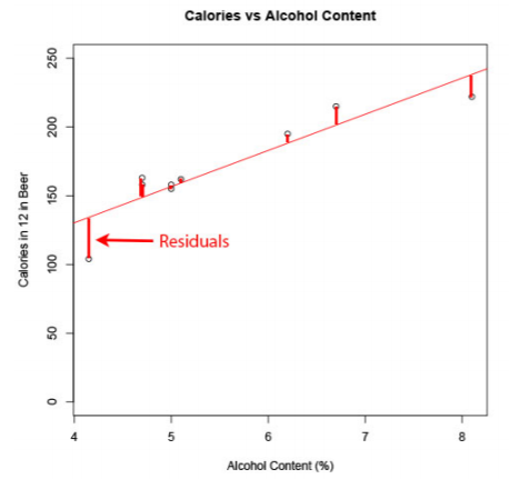
To find the equation for the linear relationship, the process of regression is used to find the line that best fits the data (sometimes called the best fitting line). The process is to draw the line through the data and then find the distances from a point to the line, which are called the residuals. The regression line is the line that makes the square of the residuals as small as possible, so the regression line is also sometimes called the least squares line. The regression line and the residuals are displayed in Figure .
Figure : Scatter Plot of Beer Data with Regression Line and Residuals
To find the regression equation (also known as best fitting line or least squares line)
Given a collection of paired sample data, the regression equation is
where the slope = and y-intercept =
The independent variable, also called the explanatory variable or predictor variable, is the x-value in the equation. The independent variable is the one that you use to predict what the other variable is. The dependent variable depends on what independent value you pick. It also responds to the explanatory variable and is sometimes called the response variable. In the alcohol content and calorie example, it makes slightly more sense to say that you would use the alcohol content on a beer to predict the number of calories in the beer.
Assumptions of the regression line:
The set of ordered pairs is a random sample from the population of all such possible pairs.
For each fixed value of x, the y-values have a normal distribution. All of the y distributions have the same variance, and for a given x-value, the distribution of y-values has a mean that lies on the least squares line. You also assume that for a fixed y, each x has its own normal distribution. This is difficult to figure out, so you can use the following to determine if you have a normal distribution.
Look to see if the scatter plot has a linear pattern.
Examine the residuals to see if there is randomness in the residuals. If there is a pattern to the residuals, then there is an issue in the data.
Notice, that the 6.50% value falls into the range of the original x-values. The processes of predicting values using an x within the range of original x-values is called interpolating. The 2.00% value is outside the range of original x-values. Using an x-value that is outside the range of the original x-values is called extrapolating. When predicting values using interpolation, you can usually feel pretty confident that that value will be close to the true value. When you extrapolate, you are not really sure that the predicted value is close to the true value. This is because when you interpolate, you know the equation that predicts, but when you extrapolate, you are not really sure that your relationship is still valid. The relationship could in fact change for different x-values.
An example of this is when you use regression to come up with an equation to predict the growth of a city, like Flagstaff, AZ. Based on analysis it was determined that the population of Flagstaff would be well over 50,000 by 1995. However, when a census was undertaken in 1995, the population was less than 50,000. This is because they extrapolated and the growth factor they were using had obviously changed from the early 1990’s. Growth factors can change for many reasons, such as employment growth, employment stagnation, disease, articles saying great place to live, etc. Realize that when you extrapolate, your predicted value may not be anywhere close to the actual value that you observe.
What does the slope mean in the context of this problem?
The calories increase 26.3 calories for every 1% increase in alcohol content.
The y-intercept in many cases is meaningless. In this case, it means that if a drink has 0 alcohol content, then it would have 25.0 calories. This may be reasonable, but remember this value is an extrapolation so it may be wrong.
Consider the residuals again. According to the data, a beer with 6.7% alcohol has 215 calories. The predicted value is 201 calories.
Residual = actual - predicted
=215 - 201
=14
This deviation means that the actual value was 14 above the predicted value. That isn’t that far off. Some of the actual values differ by a large amount from the predicted value. This is due to variability in the dependent variable. The larger the residuals the less the model explains the variability in the dependent variable. There needs to be a way to calculate how well the model explains the variability in the dependent variable. This will be explored in the next section.
The following example demonstrates the process to go through when using the formulas for finding the regression equation, though it is better to use technology. This is because if the linear model doesn’t fit the data well, then you could try some of the other models that are available through technology.
These eBooks are a prerelease and are not yet certified conformant with WCAG 2.1 AA or ADA Title II. Every page is built against an automated accessibility gate, and the published editions will meet ADA Title II requirements when they release in late September 2026. If something is unusable, please tell us.