7.3 One-Sample Test for the Mean

It is time to go back to look at the test for the mean that was introduced in section 7.1 called the z-test. In the example, you knew what the population standard deviation, $σ$ , was. What if you don’t know $σ$ ?

You could just use the sample standard deviation, s, as an approximation of $σ$ . That means the test statistic is now $\frac{\overset{―}{x} - μ}{s / \sqrt{n}}$ . Great, now you can go and find the p-value using the normal curve. Or can you? Is this new test statistic normally distributed? Actually, it is not. How is it distributed? A man named W. S. Gossett figured out what this distribution is and called it the Student’s t-distribution. There are some assumptions that must be made for this formula to be a Student’s t-distribution. These are outlined in the following theorem. Note: the t-distribution is called the Student’s t-distribution because that is the name he published under because he couldn’t publish under his own name due to employer not wanting him to publish under his own name. His employer by the way was Guinness and they didn't want competitors knowing they had a chemist working for them. It is not called the Student’s t-distribution because it is only used by students.

Theorem: If the following assumptions are met

A random sample of size n is taken.
The distribution of the random variable is normal or the sample size is 30 or more.

Then the distribution of $t = \frac{\overset{―}{x} - μ}{s / \sqrt{n}}$ is a Student’s t-distribution with $n minus 1$ degrees of freedom.

Explanation of degrees of freedom:

Recall the formula for sample standard deviation is $s = \sqrt{\frac{\sum (x - \overset{―}{x})^{2}}{n - 1}}$ . Notice the denominator is n - 1. This is the same as the degrees of freedom. This is no accident. The reason the denominator and the degrees of freedom are both n -1 comes from how the standard deviation is calculated. Remember, first you take each data value and subtract $\overset{―}{x}$ . If you add up all of these new values, you will get 0. This must happen. Since it must happen, the first n - 1 data values you have “freedom of choice”, but the nth data value, you have no freedom to choose. Hence, you have n - 1 degrees of freedom. Another way to think about it is that if you five people and five chairs, the first four people have a choice of where they are sitting, but the last person does not. They have no freedom of where to sit. Only 5 - 1 =4 people have freedom of choice.

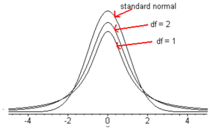
The Student’s t-distribution is a bell-shape that is more spread out than the normal distribution. There are many t-distributions, one for each different degree of freedom.

Here is a graph of the normal distribution and the Student’s t-distribution for df = 1 and df = 2.

Line chart comparing the standard normal density curve with Student’s t density curves for 1 and 2 degrees of freedom, with the t curves lower at the center and heavier in the tails. — Figure $1$ : Typical Student t-Distributions

As the degrees of freedom increases, the student’s t-distribution looks more like the normal distribution.

To find probabilities for the t-distribution, again technology can do this for you. There are many technologies out there that you can use. On the TI-83/84, the command is in the DISTR menu and is tcdf(. The syntax for this command is

tcdf(lower limit, upper limit, df)

On R: the command to find the area to the left of a t value is pt(t value, df)

Hypothesis Test for One Population Mean (t-Test)

State the random variable and the parameter in words.
x = random variable
$μ$ = mean of random variable
State the null and alternative hypotheses and the level of significance
$H_{o} : μ = μ_{o}$ , where $μ_{o}$ is the known mean
$H_{A} : μ < μ_{o}$
$H_{A} : μ > μ_{o}$ , use the appropriate one for your problem
$H_{A} : μ \neq μ_{o}$
Also, state your $α$ level here.
State and check the assumptions for a hypothesis test
1. A random sample of size n is taken.
2. The population of the random variable is normally distributed, though the t-test is fairly robust to the condition if the sample size is large. This means that if this condition isn’t met, but your sample size is quite large (over 30), then the results of the t-test are valid.
3. The population standard deviation, $σ$ , is unknown.
Find the sample statistic, test statistic, and p-value
Test Statistic:
$t = \frac{\overset{―}{x} - μ}{\frac{s}{\sqrt{n}}}$
with degrees of freedom df = n - 1
p-value:
Using TI-83/84: tcdf(lower limit, upper limit, df) Using R: pt(t value, df)
Note
Note
If $H_{A} : μ < μ_{o}$ , then lower limit is $minus 1 E 99$ and upper limit is your test statistic. If $H_{A} : μ > μ_{o}$ , then lower limit is your test statistic and the upper limit is $1 E 99$ . If $H_{A} : μ \neq μ_{o}$ , then find the p-value for $H_{A} : μ < μ_{o}$ , and multiply by 2.
Note
Note
If $H_{A} : μ < μ_{o}$ , then the command is pt(t value, df). If $H_{A} : μ > μ_{o}$ , then the command is $1 minus pt(t value, df close parenthesis$ . If $H_{A} : μ \neq μ_{o}$ , then find the p-value for $H_{A} : μ < μ_{o}$ , and multiply by 2.
This is where you write reject $H_{o}$ or fail to reject $H_{o}$ . The rule is: if the p-value < $α$ , then reject $H_{o}$ . If the p-value $\geq α$ , then fail to reject $H_{o}$ .
This is where you interpret in real world terms the conclusion to the test. The conclusion for a hypothesis test is that you either have enough evidence to show $H_{A}$ is true, or you do not have enough evidence to show $H_{A}$ is true.

How to check the assumptions of t-test:

In order for the t-test to be valid, the assumptions of the test must be true. Whenever you run a t-test, you must make sure the assumptions are true. You need to check them. Here is how you do this:

For the condition that the sample is a random sample, describe how you took the sample. Make sure your sampling technique is random.
For the condition that population of the random variable is normal, remember the process of assessing normality from chapter 6.

Example 1 test of the mean using the formula

A random sample of 20 IQ scores of famous people was taken from the website of IQ of Famous People ("IQ of famous," 2013) and a random number generator was used to pick 20 of them. The data are in Example $1$ . Do the data provide evidence at the 5% level that the IQ of a famous person is higher than the average IQ of 100?

Table $1$ : IQ Scores of Famous People
158	180	150	137	109
225	122	138	145	180
118	118	126	140	165
150	170	105	154	118

State the random variable and the parameter in words.
State the null and alternative hypotheses and the level of significance.
State and check the assumptions for a hypothesis test.
Find the sample statistic, test statistic, and p-value.
Conclusion
Interpretation

Show solution

1. x = IQ score of a famous person

$μ$ = mean IQ score of a famous person

2. $\begin{matrix} H_{o} : μ = 100 \\ H_{A} : μ > 100 \\ α = 0.05 \end{matrix}$

A random sample of 20 IQ scores was taken. This was said in the problem.
The population of IQ score is normally distributed. This was shown in Example $2$ .

4. Sample Statistic:

$\begin{matrix} \overset{―}{x} = 145.4 \\ s \approx 29.27 \end{matrix}$

Test Statistic:

$t = \frac{\overset{―}{x} - μ}{\frac{s}{\sqrt{n}}} = \frac{145.4 - 100}{\frac{29.27}{\sqrt{20}}} \approx 6.937$

p-value:

df = n - 1 = 20 - 1 = 19

TI-83/84: p-value = $tcdf (6.937, 1 E 99, 19) = 6.5 \times 10^{- 7}$

R: p-value = $1 - pt (6.937, 19) = 6.5 \times 10^{- 7}$

pt(6.937, 19)

5. Since the p-value is less than 5%, then reject $H_{o}$ .

6. There is enough evidence to show that famous people have a higher IQ than the average IQ of 100.

Example 2 test of the mean using technology

In 2011, the average life expectancy for a woman in Europe was 79.8 years. The data in Example $2$ are the life expectancies for men in European countries in 2011 ("WHO life expectancy," 2013). Do the data indicate that men’s life expectancy is less than women’s? Test at the 1% level.

Table $2$ : Life Expectancies for Men in European Countries in 2011

State the random variable and the parameter in words.
State the null and alternative hypotheses and the level of significance.
State and check the assumptions for a hypothesis test.
Find the sample statistic, test statistic, and p-value.
Conclusion
Interpretation

Show solution

1. x = life expectancy for a European man in 2011

$μ$ = mean life expectancy for European men in 2011

2. $\begin{matrix} H_{o} : μ = 79.8 years \\ H_{A} : μ < 79.8 years \\ α = 0.01 \end{matrix}$

A random sample of 53 life expectancies of European men in 2011 was taken. The data is actually all of the life expectancies for every country that is considered part of Europe by the World Health Organization. However, the information is still sample information since it is only for one year that the data was collected. It may not be a random sample, but that is probably not an issue in this case.
The distribution of life expectancies of European men in 2011 is normally distributed. To see if this condition has been met, look at the histogram, number of outliers, and the normal probability plot. (If you wish, you can look at the normal probability plot first. If it doesn’t look linear, then you may want to look at the histogram and number of outliers at this point.)

Figure

2

: Histogram for Life Expectancies of European Men in 2011

Not bell shaped

Number of outliers:

Figure

3

: Modified Box Plot for Life Expectancies of European Men in 2011

or:

IQR = 79 - 69 = 10

1.5 * IQR = 15

Q1 - 1.5 * IQR = 69 - 15 = 54

Q3 + 1.5 * IQR = 79 + 15 = 94

Outliers are numbers below 54 and above 94. There are no outliers for this data set.

Figure

4

: Normal Quantile Plot for Life Expectancies of European Men in 2011

Not linear

This population does not appear to be normally distributed. This sample is larger than 30, so it is good that the t-test is robust.

4. The calculations will be conducted using technology.

On the TI-83/84 calculator. Go into STAT and type the data into L1.

Then go into STAT and move over to TESTS. Choose T-Test. The setup for the calculator is in Figure $4$ .

Figure

5

: Setup for T-Test on TI-83/84 Calculator

Once you press ENTER on Calculate you will see the result shown in Figure $6$ .

Figure

6

: Result of T-Test on TI-83/84 Calculator

On R, the command is t.test(variable, mu = number in $H sub 0$ , alternative = "less" or "greater"), where mu = what $H sub 0$ says the mean equals, and you use less if your $H_{A}$ is less and greater if your $H_{A}$ is greater. If your $H_{A}$ is not equal to, then leave off the alternative statement. For this example, the command would be t.test(expectancy, mu=79.8, alternative = "less")

One Sample t-test

data: expectancy

t = -7.7069, df = 52, p-value = 1.853e-10

alternative hypothesis: true mean is less than 79.8

95 percent confidence interval:

-Inf 75.05357

sample estimates:

mean of x

73.73585

Most of the output you don’t need. You need the test statistic and the p-value.

The t = -7.707 is the test statistic. The p-value is $1.8534 \times 10^{- 10}$ .

5. Since the p-value is less than 1%, then reject $H_{o}$ .

6. There is enough evidence to show that the mean life expectancy for European men in 2011 was less than the mean life expectancy for European women in 2011 of 79.8 years.

Homework

Your Turn

In each problem show all steps of the hypothesis test. If some of the assumptions are not met, note that the results of the test may not be correct and then continue the process of the hypothesis test.

The Kyoto Protocol was signed in 1997, and required countries to start reducing their carbon emissions. The protocol became enforceable in February 2005. In 2004, the mean CO2 emission was 4.87 metric tons per capita. Table $3$ contains a random sample of CO2 emissions in 2010 ("CO2 emissions," 2013). Is there enough evidence to show that the mean CO2 emission is lower in 2010 than in 2004? Test at the 1% level.
Table $3$ : CO2 Emissions (in metric tons per capita) in 2010
1.36 1.42 5.93 5.36 0.06 9.11 7.32
7.93 6.72 0.78 1.80 0.20 2.27 0.28
5.86 3.46 1.46 0.14 2.62 0.79 7.48
0.86 7.84 2.87 2.45
The amount of sugar in a Krispy Kream glazed donut is 10 g. Many people feel that cereal is a healthier alternative for children over glazed donuts. Example $4$ contains the amount of sugar in a sample of cereal that is geared towards children ("Healthy breakfast story," 2013). Is there enough evidence to show that the mean amount of sugar in children’s cereal is more than in a glazed donut? Test at the 5% level.
Table $4$ : Sugar Amounts in Children's Cereal
10 14 12 9 13 13 13
11 12 15 9 10 11 3
6 12 15 12 12

The FDA regulates that fish that is consumed is allowed to contain 1.0 mg/kg of mercury. In Florida, bass fish were collected in 53 different lakes to measure the amount of mercury in the fish. The data for the average amount of mercury in each lake is in Table

5

("Multi-disciplinary niser activity," 2013). Do the data provide enough evidence to show that the fish in Florida lakes has more mercury than the allowable amount? Test at the 10% level.

Table $5$ : Average Mercury Levels (mg/kg) in Fish
1.23	1.33	0.04	0.44	1.20	0.27
0.48	0.19	0.83	0.81	0.81	0.5
0.49	1.16	0.05	0.15	0.19	0.77
1.08	0.98	0.63	0.56	0.41	0.73
0.34	0.59	0.34	0.84	0.50	0.34
0.28	0.34	0.87	0.56	0.17	0.18
0.19	0.04	0.49	1.10	0.16	0.10
0.48	0.21	0.86	0.52	0.65	0.27
0.94	0.40	0.43	0.25	0.27

Stephen Stigler determined in 1977 that the speed of light is 299,710.5 km/sec. In 1882, Albert Michelson had collected measurements on the speed of light ("Student t-distribution," 2013). His measurements are given in Example $6$ . Is there evidence to show that Michelson’s data is different from Stigler’s value of the speed of light? Test at the 5% level.
Table $6$ : Speed of Light Measurements in (km/sec)
299883 299816 299778 299796 299682
299711 299611 299599 300051 299781
299578 299796 299774 299820 299772
299696 299573 299748 299748 299797
299851 299809 299723
Table 7 contains pulse rates after running for 1 minute, collected from females who drink alcohol ("Pulse rates before," 2013). The mean pulse rate after running for 1 minute of females who do not drink is 97 beats per minute. Do the data show that the mean pulse rate of females who do drink alcohol is higher than the mean pulse rate of females who do not drink? Test at the 5% level.
Table $7$ : Pulse Rates of Woman Who Use Alcohol
176 150 150 115 129 160
120 125 89 132 120 120
68 87 88 72 77 84
92 80 60 67 59 64
88 74 68

The economic dynamism, which is the index of productive growth in dollars for countries that are designated by the World Bank as middle-income are in Table 8 ("SOCR data 2008," 2013). Countries that are considered high-income have a mean economic dynamism of 60.29. Do the data show that the mean economic dynamism of middle-income countries is less than the mean for high-income countries? Test at the 5% level.

Table $8$ : Economic Dynamism of Middle Income Countries
25.8057	37.4511	51.915	43.6952	47.8506	43.7178	58.0767
41.1648	38.0793	37.7251	39.6553	42.0265	48.6159	43.8555
49.1361	61.9281	41.9543	44.9346	46.0521	48.3652	43.6252
50.9866	59.1724	39.6282	33.6074	21.6643

In 1999, the average percentage of women who received prenatal care per country is 80.1%. Table 9 contains the percentage of woman receiving prenatal care in 2009 for a sample of countries ("Pregnant woman receiving," 2013). Do the data show that the average percentage of women receiving prenatal care in 2009 is higher than in 1999? Test at the 5% level.

Table $9$ : Percentage of Woman Receiving Prenatal Care
70.08	72.73	74.52	75.79	76.28	76.28
76.65	80.34	80.60	81.90	86.30	87.70
87.76	88.40	90.70	91.50	91.80	92.10
92.20	92.41	92.47	93.00	93.20	93.40
93.63	93.69	93.80	94.30	94.51	95.00
95.80	95.80	96.23	96.24	97.30	97.90
97.95	98.20	99.00	99.00	99.10	99.10
100.00	100.00	100.00	100.00	100.00

Maintaining your balance may get harder as you grow older. A study was conducted to see how steady the elderly is on their feet. They had the subjects stand on a force platform and have them react to a noise. The force platform then measured how much they swayed forward and backward, and the data is in Table 10 ("Maintaining balance while," 2013). Do the data show that the elderly sway more than the mean forward sway of younger people, which is 18.125 mm? Test at the 5% level.
Table $10$ : Forward/Backward Sway (in mm) of Elderly Subjects
19 30 20 19 29 25 21 24 50

Answer

For all hypothesis tests, just the conclusion is given. See solutions for the entire answer.

1. Fail to reject Ho.

3. Fail to reject Ho.

5. Fail to reject Ho.

7. Reject Ho.

Data Sources:

Australian Human Rights Commission, (1996). Indigenous deaths in custody 1989 - 1996. Retrieved from website: www.humanrights.gov.au/public...deaths-custody

CDC features - new data on autism spectrum disorders. (2013, November 26). Retrieved from www.cdc.gov/features/countingautism/

Center for Disease Control and Prevention, Prevalence of Autism Spectrum Disorders - Autism and Developmental Disabilities Monitoring Network. (2008). Autism and developmental disabilities monitoring network-2012. Retrieved from website: www.cdc.gov/ncbddd/autism/doc...nityReport.pdf

CO2 emissions. (2013, November 19). Retrieved from http://data.worldbank.org/indicator/EN.ATM.CO2E.PC

Federal Trade Commission, (2008). Consumer fraud and identity theft complaint data: January-December 2007. Retrieved from website: www.ftc.gov/opa/2008/02/fraud.pdf

Gallup news service. (2013, November 7-10). Retrieved from www.gallup.com/file/poll/1658...acy_131115.pdf

Healthy breakfast story. (2013, November 16). Retrieved from lib.stat.cmu.edu/DASL/Stories...Breakfast.html

IQ of famous people. (2013, November 13). Retrieved from http://www.kidsiqtestcenter.com/IQ-famous-people.html

Maintaining balance while concentrating. (2013, September 25). Retrieved from http://www.statsci.org/data/general/balaconc.html

Morgan Gallup poll on unemployment. (2013, September 26). Retrieved from http://www.statsci.org/data/oz/gallup.html

Multi-disciplinary niser activity - mercury in bass. (2013, November 16). Retrieved from http://gozips.uakron.edu/~nmimoto/pa.../MercuryInBass - description.txt

Pregnant woman receiving prenatal care. (2013, October 14). Retrieved from http://data.worldbank.org/indicator/SH.STA.ANVC.ZS

SOCR data 2008 world countries rankings. (2013, November 16). Retrieved from http://wiki.stat.ucla.edu/socr/index...ntriesRankings

Student t-distribution. (2013, November 25). Retrieved from lib.stat.cmu.edu/DASL/Stories/student.html

WHO life expectancy. (2013, September 19). Retrieved from www.who.int/gho/mortality_bur...n_trends/en/in dex.html

1.36	1.42	5.93	5.36	0.06	9.11	7.32
7.93	6.72	0.78	1.80	0.20	2.27	0.28
5.86	3.46	1.46	0.14	2.62	0.79	7.48
0.86	7.84	2.87	2.45

299883	299816	299778	299796	299682
299711	299611	299599	300051	299781
299578	299796	299774	299820	299772
299696	299573	299748	299748	299797
299851	299809	299723

Table $7$ : Pulse Rates of Woman Who Use Alcohol
176	150	150	115	129	160
120	125	89	132	120	120
68	87	88	72	77	84
92	80	60	67	59	64
88	74	68