7.1 Basics of Hypothesis Testing

To understand the process of a hypothesis tests, you need to first have an understanding of what a hypothesis is, which is an educated guess about a parameter. Once you have the hypothesis, you collect data and use the data to make a determination to see if there is enough evidence to show that the hypothesis is true. However, in hypothesis testing you actually assume something else is true, and then you look at your data to see how likely it is to get an event that your data demonstrates with that assumption. If the event is very unusual, then you might think that your assumption is actually false. If you are able to say this assumption is false, then your hypothesis must be true. This is known as a proof by contradiction. You assume the opposite of your hypothesis is true and show that it can’t be true. If this happens, then your hypothesis must be true. All hypothesis tests go through the same process. Once you have the process down, then the concept is much easier. It is easier to see the process by looking at an example. Concepts that are needed will be detailed in this example.

Example 1 basics of hypothesis testing

Suppose a manufacturer of the XJ35 battery claims the mean life of the battery is 500 days with a standard deviation of 25 days. You are the buyer of this battery and you think this claim is inflated. You would like to test your belief because without a good reason you can’t get out of your contract.

What do you do?

Show solution

Well first, you should know what you are trying to measure. Define the random variable.

Let x = life of a XJ35 battery

Now you are not just trying to find different x values. You are trying to find what the true mean is. Since you are trying to find it, it must be unknown. You don’t think it is 500 days. If you did, you wouldn’t be doing any testing. The true mean, $μ$ , is unknown. That means you should define that too.

Let $μ$ = mean life of a XJ35 battery

Now what?

You may want to collect a sample. What kind of sample?

You could ask the manufacturers to give you batteries, but there is a chance that there could be some bias in the batteries they pick. To reduce the chance of bias, it is best to take a random sample.

How big should the sample be?

A sample of size 30 or more means that you can use the central limit theorem. Pick a sample of size 30.

Example $1$ contains the data for the sample you collected:

Table $1$ : Data on Battery Life
491	485	503	492	282	490
489	495	497	487	493	480
483	504	501	486	478	492
482	502	485	503	497	500
488	475	478	490	487	486

Now what should you do? Looking at the data set, you see some of the times are above 500 and some are below. But looking at all of the numbers is too difficult. It might be helpful to calculate the mean for this sample.

The sample mean is $x ― equals 490$ days. Looking at the sample mean, one might think that you are right. However, the standard deviation and the sample size also plays a role, so maybe you are wrong.

Before going any farther, it is time to formalize a few definitions.

You have a guess that the mean life of a battery is less than 500 days. This is opposed to what the manufacturer claims. There really are two hypotheses, which are just guesses here – the one that the manufacturer claims and the one that you believe. It is helpful to have names for them.

Definition

Alternate Hypothesis: what you want to prove. This is what you want to accept as true when you reject the null hypothesis. There are two symbols that are commonly used for the alternative hypothesis: $H_{A}$ or $H_{I}$ . The symbol $H_{A}$ will be used in this book.

In general, the hypotheses look something like this:

$H_{o} : μ = μ_{o}$

$H_{A} : μ < μ_{o}$

where $μ_{o}$ just represents the value that the claim says the population mean is actually equal to.

Also, $H_{A}$ can be less than, greater than, or not equal to.

For this problem:

$H sub o: μ equals 500$ days, since the manufacturer says the mean life of a battery is 500 days.

$H sub A: μ less than 500$ days, since you believe that the mean life of the battery is less than 500 days.

Now back to the mean. You have a sample mean of 490 days. Is this small enough to believe that you are right and the manufacturer is wrong? How small does it have to be?

If you calculated a sample mean of 235, you would definitely believe the population mean is less than 500. But even if you had a sample mean of 435 you would probably believe that the true mean was less than 500. What about 475? Or 483? There is some point where you would stop being so sure that the population mean is less than 500. That point separates the values of where you are sure or pretty sure that the mean is less than 500 from the area where you are not so sure. How do you find that point?

Well it depends on how much error you want to make. Of course you don’t want to make any errors, but unfortunately that is unavoidable in statistics. You need to figure out how much error you made with your sample. Take the sample mean, and find the probability of getting another sample mean less than it, assuming for the moment that the manufacturer is right. The idea behind this is that you want to know what is the chance that you could have come up with your sample mean even if the population mean really is 500 days.

You want to find $P (\overset{―}{x} < 490 | H_{o} is true) = P (\overset{―}{x} < 490 | μ = 500)$

To compute this probability, you need to know how the sample mean is distributed. Since the sample size is at least 30, then you know the sample mean is approximately normally distributed. Remember $μ_{\overset{―}{x}} = μ$ and $σ_{\overset{―}{x}} = \frac{σ}{\sqrt{n}}$

A picture is always useful.

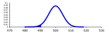
A smooth normal density curve centered at 500 peaks near 0.09 and approaches zero by about 480 and 520. — Figure $1$

Before calculating the probability, it is useful to see how many standard deviations away from the mean the sample mean is. Using the formula for the z-score from chapter 6, you find

$z = \frac{\overset{―}{x} - μ_{o}}{σ / \sqrt{n}} = \frac{490 - 500}{25 / \sqrt{30}} = - 2.19$

This sample mean is more than two standard deviations away from the mean. That seems pretty far, but you should look at the probability too.

On TI-83/84:

$P (\overset{―}{x} < 490 | μ = 500) = normalcdf (- 1 E 99, 490, 500, 25 \div \sqrt{30}) \approx 0.0142$

On R:

$P (\overset{―}{x} < 490 μ = 500) = pnorm (490, 500, 25 / sqrt (30)) \approx 0.0142$

pnorm(490, 500, 25/sqrt(30))

There is a 1.42% chance that you could find a sample mean less than 490 when the population mean is 500 days. This is really small, so the chances are that the assumption that the population mean is 500 days is wrong, and you can reject the manufacturer’s claim. But how do you quantify really small? Is 5% or 10% or 15% really small? How do you decide?

Before you answer that question, a couple more definitions are needed.

Now, how small is small enough? To answer that, you really want to know the types of errors you can make.

There are actually only two errors that can be made. The first error is if you say that $H_{o}$ is false, when in fact it is true. This means you reject $H_{o}$ when $H_{o}$ was true. The second error is if you say that $H_{o}$ is true, when in fact it is false. This means you fail to reject $H_{o}$ when $H_{o}$ is false. The following table organizes this for you:

Type of errors:

Table $2$ : Types of Errors
	$H_{o}$ true	$H_{o}$ false
Reject $H_{o}$	Type 1 error	No error
Fail to reject $H_{o}$	No error	Type II error

Thus

Since these are the errors, then one can define the probabilities attached to each error.

$α$ is also called the level of significance.

Another common concept that is used is Power = $1 minus β$ .

Now there is a relationship between $α$ and $β$ . They are not complements of each other. How are they related?

If $α$ increases that means the chances of making a type I error will increase. It is more likely that a type I error will occur. It makes sense that you are less likely to make type II errors, only because you will be rejecting $H_{o}$ more often. You will be failing to reject $H_{o}$ less, and therefore, the chance of making a type II error will decrease. Thus, as $α$ increases, $β$ will decrease, and vice versa. That makes them seem like complements, but they aren’t complements. What gives? Consider one more factor – sample size.

Consider if you have a larger sample that is representative of the population, then it makes sense that you have more accuracy then with a smaller sample. Think of it this way, which would you trust more, a sample mean of 490 if you had a sample size of 35 or sample size of 350 (assuming a representative sample)? Of course the 350 because there are more data points and so more accuracy. If you are more accurate, then there is less chance that you will make any error. By increasing the sample size of a representative sample, you decrease both $α$ and $β$ .

Summary of all of this:

For a certain sample size, n, if $α$ increases, $β$ decreases.
For a certain level of significance, $α$ , if n increases, $β$ decreases.

Now how do you find $α$ and $β$ ? Well $α$ is actually chosen. There are only three values that are usually picked for $α$ : 0.01, 0.05, and 0.10. $β$ is very difficult to find, so usually it isn’t found. If you want to make sure it is small you take as large of a sample as you can afford provided it is a representative sample. This is one use of the Power. You want $β$ to be small and the Power of the test is large. The Power word sounds good.

Which pick of $α$ do you pick? Well that depends on what you are working on. Remember in this example you are the buyer who is trying to get out of a contract to buy these batteries. If you create a type I error, you said that the batteries are bad when they aren’t, most likely the manufacturer will sue you. You want to avoid this. You might pick $α$ to be 0.01. This way you have a small chance of making a type I error. Of course this means you have more of a chance of making a type II error. No big deal right? What if the batteries are used in pacemakers and you tell the person that their pacemaker’s batteries are good for 500 days when they actually last less, that might be bad. If you make a type II error, you say that the batteries do last 500 days when they last less, then you have the possibility of killing someone. You certainly do not want to do this. In this case you might want to pick $α$ as 0.10. If both errors are equally bad, then pick $α$ as 0.05.

The above discussion is why the choice of $α$ depends on what you are researching. As the researcher, you are the one that needs to decide what $α$ level to use based on your analysis of the consequences of making each error is.

The main thing is to always pick the $α$ before you collect the data and start the test.

The above discussion was long, but it is really important information. If you don’t know what the errors of the test are about, then there really is no point in making conclusions with the tests. Make sure you understand what the two errors are and what the probabilities are for them.

Now it is time to go back to the example and put this all together. This is the basic structure of testing a hypothesis, usually called a hypothesis test. Since this one has a test statistic involving z, it is also called a z-test. And since there is only one sample, it is usually called a one-sample z-test.

Example 2 battery example revisited

State the random variable and the parameter in words.
State the null and alternative hypothesis and the level of significance.
State and check the assumptions for a hypothesis test.
1. A random sample of size n is taken.
2. The population standard deviation is known.
3. The sample size is at least 30 or the population of the random variable is normally distributed.
Find the sample statistic, test statistic, and p-value.
Conclusion
Interpretation

Show solution

1. x = life of battery

$μ$ = mean life of a XJ35 battery

2. $H sub o: μ equals 500$ days

$H sub A: μ less than 500$ days

$α equals 0.10$ (from above discussion about consequences)

3. Every hypothesis has some assumptions that be met to make sure that the results of the hypothesis are valid. The assumptions are different for each test. This test has the following assumptions.

This occurred in this example, since it was stated that a random sample of 30 battery lives were taken.
This is true, since it was given in the problem.
The sample size was 30, so this condition is met.

4. The test statistic depends on how many samples there are, what parameter you are testing, and assumptions that need to be checked. In this case, there is one sample and you are testing the mean. The assumptions were checked above.

Sample statistic:

$x ― equals 490$

Test statistic:

$z = \frac{\overset{―}{x} - μ_{o}}{σ / \sqrt{n}} = \frac{490 - 500}{25 / \sqrt{30}} = - 2.19$

p-value:

Figure

2

Using TI-83/84:

$P (\overset{―}{x} < 490 | μ = 500) = normalcdf (- 1 E 99, 490, 500, 25 / \sqrt{30}) \approx 0.0142$

Using R:

$P (\overset{―}{x} < 490 | μ = 500) = pnorm (490, 500, 25 / sqrt (30)) \approx 0.0142$

5. Now what? Well, this p-value is 0.0142. This is a lot smaller than the amount of error you would accept in the problem - $α$ = 0.10. That means that finding a sample mean less than 490 days is unusual to happen if $H_{o}$ is true. This should make you think that $H_{o}$ is not true. You should reject $H_{o}$ .

6. Since you rejected $H_{o}$ , what does this mean in the real world? That is what goes in the interpretation. Since you rejected the claim by the manufacturer that the mean life of the batteries is 500 days, then you now can believe that your hypothesis was correct. In other words, there is enough evidence to show that the mean life of the battery is less than 500 days.

Now that you know that the batteries last less than 500 days, should you cancel the contract? Statistically, there is evidence that the batteries do not last as long as the manufacturer says they should. However, based on this sample there are only ten days less on average that the batteries last. There may not be practical significance in this case. Ten days do not seem like a large difference. In reality, if the batteries are used in pacemakers, then you would probably tell the patient to have the batteries replaced every year. You have a large buffer whether the batteries last 490 days or 500 days. It seems that it might not be worth it to break the contract over ten days. What if the 10 days was practically significant? Are there any other things you should consider? You might look at the business relationship with the manufacturer. You might also look at how much it would cost to find a new manufacturer. These are also questions to consider before making any changes. What this discussion should show you is that just because a hypothesis has statistical significance does not mean it has practical significance. The hypothesis test is just one part of a research process. There are other pieces that you need to consider.

That’s it. That is what a hypothesis test looks like. All hypothesis tests are done with the same six steps. Those general six steps are outlined below.

State the random variable and the parameter in words. This is where you are defining what the unknowns are in this problem.
x = random variable
$μ$ = mean of random variable, if the parameter of interest is the mean. There are other parameters you can test, and you would use the appropriate symbol for that parameter.
State the null and alternative hypotheses and the level of significance
$H_{o} : μ = μ_{o}$ , where $μ_{o}$ is the known mean
$H_{A} : μ < μ_{o}$
$H_{A} : μ > μ_{o}$ , use the appropriate one for your problem
$H_{A} : μ \neq μ_{o}$
Also, state your $α$ level here.
State and check the assumptions for a hypothesis test.
Each hypothesis test has its own assumptions. They will be stated when the different hypothesis tests are discussed.
Find the sample statistic, test statistic, and p-value.
This depends on what parameter you are working with, how many samples, and the assumptions of the test. The p-value depends on your $H_{A}$ . If you are doing the $H_{A}$ with the less than, then it is a left-tailed test, and you find the probability of being in that left tail. If you are doing the $H_{A}$ with the greater than, then it is a right-tailed test, and you find the probability of being in the right tail. If you are doing the $H_{A}$ with the not equal to, then you are doing a two-tail test, and you find the probability of being in both tails. Because of symmetry, you could find the probability in one tail and double this value to find the probability in both tails.
Conclusion
This is where you write reject $H_{o}$ or fail to reject $H_{o}$ . The rule is: if the p-value < $α$ , then reject $H_{o}$ . If the p-value $\geq α$ , then fail to reject $H_{o}$ .
Interpretation
This is where you interpret in real world terms the conclusion to the test. The conclusion for a hypothesis test is that you either have enough evidence to show $H_{A}$ is true, or you do not have enough evidence to show $H_{A}$ is true.

Sorry, one more concept about the conclusion and interpretation. First, the conclusion is that you reject $H_{o}$ or you fail to reject $H_{o}$ . Why was it said like this? It is because you never accept the null hypothesis. If you wanted to accept the null hypothesis, then why do the test in the first place? In the interpretation, you either have enough evidence to show $H_{A}$ is true, or you do not have enough evidence to show $H_{A}$ is true. You wouldn’t want to go to all this work and then find out you wanted to accept the claim. Why go through the trouble? You always want to show that the alternative hypothesis is true. Sometimes you can do that and sometimes you can’t. It doesn’t mean you proved the null hypothesis; it just means you can’t prove the alternative hypothesis. Here is an example to demonstrate this.

Example 3 conclusion in hypothesis tests

In the U.S. court system a jury trial could be set up as a hypothesis test. To really help you see how this works, let’s use OJ Simpson as an example. In the court system, a person is presumed innocent until he/she is proven guilty, and this is your null hypothesis. OJ Simpson was a football player in the 1970s. In 1994 his ex-wife and her friend were killed. OJ Simpson was accused of the crime, and in 1995 the case was tried. The prosecutors wanted to prove OJ was guilty of killing his wife and her friend, and that is the alternative hypothesis

Show solution

$H sub 0$ : OJ is innocent of killing his wife and her friend

$H_{A}$ : OJ is guilty of killing his wife and her friend

In this case, a verdict of not guilty was given. That does not mean that he is innocent of this crime. It means there was not enough evidence to prove he was guilty. Many people believe that OJ was guilty of this crime, but the jury did not feel that the evidence presented was enough to show there was guilt. The verdict in a jury trial is always guilty or not guilty!

The same is true in a hypothesis test. There is either enough or not enough evidence to show that alternative hypothesis. It is not that you proved the null hypothesis true.

When identifying hypothesis, it is important to state your random variable and the appropriate parameter you want to make a decision about. If count something, then the random variable is the number of whatever you counted. The parameter is the proportion of what you counted. If the random variable is something you measured, then the parameter is the mean of what you measured. (Note: there are other parameters you can calculate, and some analysis of those will be presented in later chapters.)

Example 4 stating hypotheses

Identify the hypotheses necessary to test the following statements:

The average salary of a teacher is more than $30,000.
The proportion of students who like math is less than 10%.
The average age of students in this class differs from 21.

Show solution

a. x = salary of teacher

$μ$ = mean salary of teacher

The guess is that $μ greater than $ 30, 000$ and that is the alternative hypothesis.

The null hypothesis has the same parameter and number with an equal sign.

$H sub 0: μ equals $ 30, 000; H sub A: μ greater than $ 30, 000$

b. x = number of students who like math

p = proportion of students who like math

The guess is that p < 0.10 and that is the alternative hypothesis.

$H sub 0: p equals 0.10; H sub A: p less than 0.10$

c. x = age of students in this class

$μ$ = mean age of students in this class

The guess is that $μ not equal to 21$ and that is the alternative hypothesis.

$H sub 0: μ equals 21; H sub A: μ not equal to 21$

Example 5 Stating Type I and II Errors and Picking Level of Significance

The plant-breeding department at a major university developed a new hybrid raspberry plant called YumYum Berry. Based on research data, the claim is made that from the time shoots are planted 90 days on average are required to obtain the first berry with a standard deviation of 9.2 days. A corporation that is interested in marketing the product tests 60 shoots by planting them and recording the number of days before each plant produces its first berry. The sample mean is 92.3 days. The corporation wants to know if the mean number of days is more than the 90 days claimed. State the type I and type II errors in terms of this problem, consequences of each error, and state which level of significance to use.
A concern was raised in Australia that the percentage of deaths of Aboriginal prisoners was higher than the percent of deaths of non-indigenous prisoners, which is 0.27%. State the type I and type II errors in terms of this problem, consequences of each error, and state which level of significance to use.

Show solution

a. x = time to first berry for YumYum Berry plant

$μ$ = mean time to first berry for YumYum Berry plant

$H sub 0: μ equals 90; H sub A: μ greater than 90$

Type I Error: If the corporation does a type I error, then they will say that the plants take longer to produce than 90 days when they don’t. They probably will not want to market the plants if they think they will take longer. They will not market them even though in reality the plants do produce in 90 days. They may have loss of future earnings, but that is all.

Type II error: The corporation do not say that the plants take longer then 90 days to produce when they do take longer. Most likely they will market the plants. The plants will take longer, and so customers might get upset and then the company would get a bad reputation. This would be really bad for the company.

Level of significance: It appears that the corporation would not want to make a type II error. Pick a 10% level of significance, $α equals 0.10$ .

b. x = number of Aboriginal prisoners who have died

p = proportion of Aboriginal prisoners who have died

$H sub o: p equals 0.27; H sub A: p greater than 0.27$

Type I error: Rejecting that the proportion of Aboriginal prisoners who died was 0.27%, when in fact it was 0.27%. This would mean you would say there is a problem when there isn’t one. You could anger the Aboriginal community, and spend time and energy researching something that isn’t a problem.

Type II error: Failing to reject that the proportion of Aboriginal prisoners who died was 0.27%, when in fact it is higher than 0.27%. This would mean that you wouldn’t think there was a problem with Aboriginal prisoners dying when there really is a problem. You risk causing deaths when there could be a way to avoid them.

Level of significance: It appears that both errors may be issues in this case. You wouldn’t want to anger the Aboriginal community when there isn’t an issue, and you wouldn’t want people to die when there may be a way to stop it. It may be best to pick a 5% level of significance, $α equals 0.05$ .

Homework

Your Turn

For the problems in this section, a question is being asked. This is to help you understand what the hypotheses are. You are not to run any hypothesis tests and come up with any conclusions in this section.

Eyeglassomatic manufactures eyeglasses for different retailers. They test to see how many defective lenses they made in a given time period and found that 11% of all lenses had defects of some type. Looking at the type of defects, they found in a three-month time period that out of 34,641 defective lenses, 5865 were due to scratches. Are there more defects from scratches than from all other causes? State the random variable, population parameter, and hypotheses.
According to the February 2008 Federal Trade Commission report on consumer fraud and identity theft, 23% of all complaints in 2007 were for identity theft. In that year, Alaska had 321 complaints of identity theft out of 1,432 consumer complaints ("Consumer fraud and," 2008). Does this data provide enough evidence to show that Alaska had a lower proportion of identity theft than 23%? State the random variable, population parameter, and hypotheses.
The Kyoto Protocol was signed in 1997, and required countries to start reducing their carbon emissions. The protocol became enforceable in February 2005. In 2004, the mean CO2 emission was 4.87 metric tons per capita. Is there enough evidence to show that the mean CO2 emission is lower in 2010 than in 2004? State the random variable, population parameter, and hypotheses.
The FDA regulates that fish that is consumed is allowed to contain 1.0 mg/kg of mercury. In Florida, bass fish were collected in 53 different lakes to measure the amount of mercury in the fish. The data for the average amount of mercury in each lake is in Table 5 of Section 7.3 ("Multi-disciplinary niser activity," 2013). Do the data provide enough evidence to show that the fish in Florida lakes has more mercury than the allowable amount? State the random variable, population parameter, and hypotheses.
Eyeglassomatic manufactures eyeglasses for different retailers. They test to see how many defective lenses they made in a given time period and found that 11% of all lenses had defects of some type. Looking at the type of defects, they found in a three-month time period that out of 34,641 defective lenses, 5865 were due to scratches. Are there more defects from scratches than from all other causes? State the type I and type II errors in this case, consequences of each error type for this situation from the perspective of the manufacturer, and the appropriate alpha level to use. State why you picked this alpha level.
According to the February 2008 Federal Trade Commission report on consumer fraud and identity theft, 23% of all complaints in 2007 were for identity theft. In that year, Alaska had 321 complaints of identity theft out of 1,432 consumer complaints ("Consumer fraud and," 2008). Does this data provide enough evidence to show that Alaska had a lower proportion of identity theft than 23%? State the type I and type II errors in this case, consequences of each error type for this situation from the perspective of the state of Arizona, and the appropriate alpha level to use. State why you picked this alpha level.
The Kyoto Protocol was signed in 1997, and required countries to start reducing their carbon emissions. The protocol became enforceable in February 2005. In 2004, the mean CO2 emission was 4.87 metric tons per capita. Is there enough evidence to show that the mean CO2 emission is lower in 2010 than in 2004? State the type I and type II errors in this case, consequences of each error type for this situation from the perspective of the agency overseeing the protocol, and the appropriate alpha level to use. State why you picked this alpha level.
The FDA regulates that fish that is consumed is allowed to contain 1.0 mg/kg of mercury. In Florida, bass fish were collected in 53 different lakes to measure the amount of mercury in the fish. The data for the average amount of mercury in each lake is in Table 5 of Section 7.3 ("Multi-disciplinary niser activity," 2013). Do the data provide enough evidence to show that the fish in Florida lakes has more mercury than the allowable amount? State the type I and type II errors in this case, consequences of each error type for this situation from the perspective of the FDA, and the appropriate alpha level to use. State why you picked this alpha level.

Answer

1. $H sub o: p equals 0.11, H sub A: p greater than 0.11$

3. $H sub o: μ equals 4.87 metric tons per capita, H sub A: μ less than 4.87 metric tons per capita$

5. See solutions

7. See solutions

491	485	503	492	282	490
489	495	497	487	493	480
483	504	501	486	478	492
482	502	485	503	497	500
488	475	478	490	487	486

491	485	503	492	282	490
489	495	497	487	493	480
483	504	501	486	478	492
482	502	485	503	497	500
488	475	478	490	487	486

491	485	503	492	282	490
489	495	497	487	493	480
483	504	501	486	478	492
482	502	485	503	497	500
488	475	478	490	487	486