Binomial distribution The discrete binomial distribution is defined to be the probability of achieving successes in a given events where each event has a given probability of success.
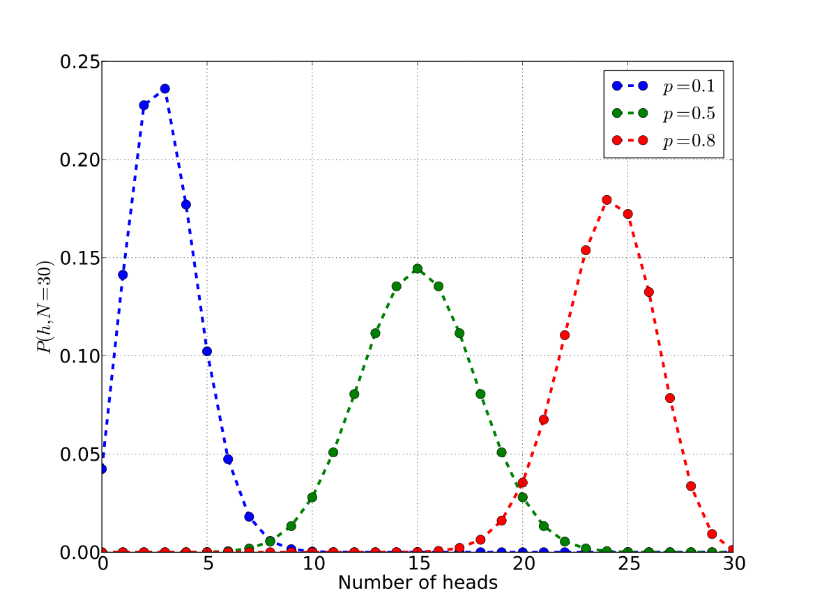
Figure C.4. Probability of getting heads in 30 flips given a possible unfair coin. One coin has , where the maximum is for 3 heads (or 1/10 of the 30 flips), but 2 heads is nearly as likely. Another has , and is the fair coin considered earlier with a maximum at 15 heads (or 1/2 of the 30 flips). Finally, another coin shown as where 24 heads (or 8/10 of the 30 flips) is maximum.
Although it may look like a Beta, the binomial distribution is used to find the best estimate for the number of successes, , given the number of events, , and the probability of the success of a single event, .
Adapted from Statistical Inference for Everyone, by Brian Blais (Bryant University), licensed under CC BY-SA 4.0 (dual-licensed under the GNU FDL 1.2 or later; this adaptation uses the CC BY-SA grant). Changes were made; this adaptation is distributed under the same license. License: CC-BY-SA-4.0.
These eBooks are a prerelease and are not yet certified conformant with WCAG 2.1 AA or ADA Title II. Every page is built against an automated accessibility gate, and the published editions will meet ADA Title II requirements when they release in late September 2026. If something is unusable, please tell us.