
10.3 Multiple regression
In order to control for a variable that may be affecting our result, we simply expand our linear model, including slopes (also called coefficients) for each of the different variables. Once we do this, visualization becomes challenging because we move into three or more dimensions. Instead of for the slope, the multiple slopes are typically labeled with the greek letter and numbered, such as etc... The intercept is then labeled . The model structure, however, is the same, and can be written
where the different , , etc... denote different variables. For the example of the SAT scores, we might have
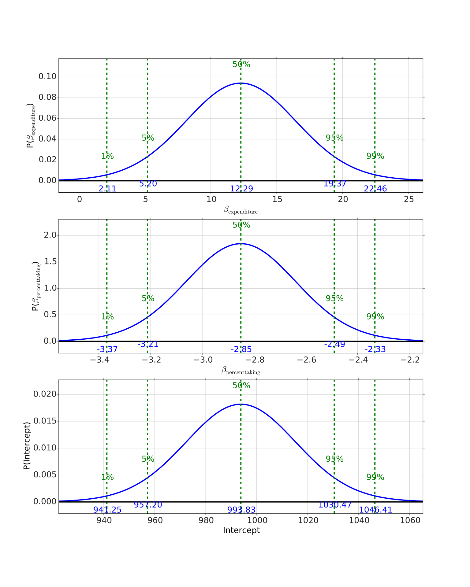
where is a variable representing the percent of students taking the exam. Including this variable gives the posterior distributions shown in Figure 10.8. Notice that the effect of expenditure is both statistically significant and positive. We can interpret the values in the following way.
- For each $1000 more spent per pupil the total SAT score increases on average by 12.29.
- For each percent increase in students taking the SAT, the total SAT score decreases on average by 2.29.
Have we controlled for all of the effects? Perhaps not! This is where the ingenuity and expertise of the person analyzing the problem comes into play.
Adapted from Statistical Inference for Everyone, by Brian Blais (Bryant University), licensed under CC BY-SA 4.0 (dual-licensed under the GNU FDL 1.2 or later; this adaptation uses the CC BY-SA grant). Changes were made; this adaptation is distributed under the same license. License: CC-BY-SA-4.0.