5.4 Psychic Octopi

There was a German octopus named Paul¹ who was claimed to be psychic during his lifetime. He was given this designation because he was supposedly able to pick the result of World Cup matches before they occurred. His impressive results, across 2 years, shown in Figure 5.2 can be summarized as follows:

$d a t a ≡ 12 out of 14 correctly predicted$

Table of Paul the Octopus's six predictions at UEFA Euro 2008. For each match: the teams, stage, date, Paul's prediction and the result. He picked Germany every time. Four are marked Correct — Germany 2-0 Poland, Austria 0-1 Germany, Portugal 2-3 Germany and Germany 3-2 Turkey — and two Incorrect: Croatia 2-1 Germany and the final, Germany 0-1 Spain. Four of six predictions correct. — **Figure 5.2.** The full results of the predictions of Paul the Octopus, the match data is from en.wikipedia.org/wiki/Psychic_octopus; the tables here are redrawn for this edition.

Table of Paul the Octopus's eight predictions at the 2010 FIFA World Cup. For each match: the teams, stage, date, prediction and result. Every one is marked Correct, including picking Serbia to beat Germany, Spain to beat Germany in the semi-final, and Spain to win the final 1-0 over the Netherlands. Eight of eight predictions correct.

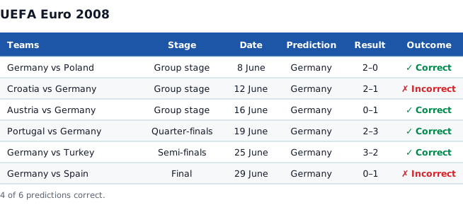
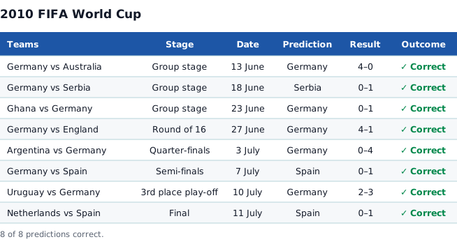
The question we have to ask is, is this data strong evidence for a psychic octopus? In order to have a well-posed problem we need the following three components:

a set of hypotheses, or models, to compare - we need at least two, otherwise the question is meaningless
for each model, an equation denoting the likelihood, or in other words, how probable is the data given the particular model
a specification of the prior probability, or in other words, how likely was our model before we saw the data

Making a Well Posed Problem

We are interested in the probability of this octopus being psychic, given this data, or

$\begin{matrix} P (p s y c h i c | d a t a) \end{matrix}$

which really is an example of a model comparison, or hypothesis testing. In any kind of model comparison, we need to have multiple models to compare to in order to proceed. The models we consider constrain the problem, and define which ideas we are willing to consider. To be specific, as a first step, let's consider the following two models

$\begin{matrix} H : = {Paul is psychic} \\ R : = {Paul is completely random, like a coin flip} \end{matrix}$

The next step is to be able to assign probabilities from these models. It is easy for the random hypothesis

$\begin{matrix} P (correct prediction | R) = 0.5 \\ P (incorrect prediction | R) = 0.5 \end{matrix}$

What does it mean to be psychic? What is the probability of getting a correct result if you are psychic? According to James Randi² many of the psychics and dowsers claim 100% accuracy in their predictions before they are tested. However this would mean a single wrong answer would drive the probability of that model to zero: a perfect predictor cannot, logically, make any mistakes. For our case here, we choose to be generous to the psychic and allow for a reasonable failure rate, using 90% as our accuracy, thus

$\begin{matrix} P (correct prediction | H) = 0.9 \\ P (incorrect prediction | H) = 0.1 \end{matrix}$

Specifying the prior probability of these two models is a bit more challenging. It seems reasonable to assign a small prior probability to a psychic octopus - how many psychic octopi have you ever encountered? A small, but still quite conservative value, would be 1/100, so we have for the two models:

$\begin{matrix} P (H) = 1 / 100 \\ P (R) = 99 / 100 \end{matrix}$

The First Model Comparison

Now that we've set up the problem, we can apply the Bayes' Recipe

Try it in XYZ Crunch

Paul's two likelihoods, before the priors go in

Both models predict the same data with a binomial, differing only in p. Subtract consecutive cumulative lookups to get the probability of exactly 12 correct in 14: the psychic model (p = 0.9) gives 0.415371 - 0.158360 = 0.257011, and times the 1/100 prior that is the book's 0.00257. The random model (p = 0.5) gives 0.999084 - 0.993530 = 0.005554, and times the 99/100 prior that is 0.00550, the book's 0.00549. Notice the psychic model predicts the DATA far better and still loses: the prior does the work.

Specify the prior probabilities for the models being considered
$\begin{matrix} P (H) = 1 / 100 \\ P (R) = 99 / 100 \end{matrix}$
Write the top of Bayes' Rule for all models being considered
$\begin{matrix} P (H | d a t a = 12 out of 14) \sim P (d a t a = 12 out of 14 | H) P (H) \\ P (R | d a t a = 12 out of 14) \sim P (d a t a = 12 out of 14 | R) P (R) \end{matrix}$
where we are using the symbol $∼$ to denote proportionality or related to. Essentially, by calculating the top of Bayes' Rule first, the numbers are not equal to the final (i.e. posterior) probabilities but must be rescaled to make sure that they add up to 1. This is done in the final step. Up until that rescaling, we use the symbol $∼$ and think of it as related to.
Put in the likelihood and prior values
$\begin{matrix} P (H | d a t a = 12 out of 14) \sim (\binom{14}{12}) {0.9}^{12} {0.1}^{14 - 12} \times \frac{1}{100} \\ = 0.00257 \\ P (R | d a t a = 12 out of 14) \sim (\binom{14}{12}) {0.5}^{12} {0.5}^{14 - 12} \times \frac{99}{100} \\ = 0.00549 \end{matrix}$
Add these values for all models
$\begin{matrix} K = 0.00257 + 0.00549 = 0.00806 \end{matrix}$
Divide each of the values by this sum, $K$ , to get the final probabilities
$\begin{matrix} P (H | d a t a) = \frac{0.00257}{0.00806} = 0.32 \\ P (R | d a t a) = \frac{0.00549}{0.00806} = 0.68 \end{matrix}$

and the psychic loses! We continue this problem discussing the potential anti-psychic bias in the presentation of the problem.

Furthering the Comparison

Typically, a person who is supportive of psychic phenomena would choose a prior for our psychic hypothesis ( $H$ ) that would be at least as large as the prior for the random hypothesis ( $R$ ). In this case, the (posterior) probability of the octopus being psychic given the data of 12 correct out of 14 would be much higher. After “ruling out” the random octopus hypothesis, we'd be left with psychic. But is that all that is really left? No, and the analysis is easy to do.

Once presented with the success of Paul, most people instantly are suspicious of random octopus, but don't adopt psychic octopus as the answer. Perhaps the keepers, being German, biased the data taking a little bit. Perhaps the octopus chose flags with bright yellow stripes. Notice that each of these cases still results in similar data - the octopus would have gotten 11 or 12 out of 14, but the prior probability of these cases should be much higher than psychic, even if lower than random. We leave it as an exercise to perform the calculation in this case, but it is directly parallel to the Nines deck example of Section 4.3 on page 102.

Adapted from Statistical Inference for Everyone, by Brian Blais (Bryant University), licensed under CC BY-SA 4.0 (dual-licensed under the GNU FDL 1.2 or later; this adaptation uses the CC BY-SA grant). Changes were made; this adaptation is distributed under the same license. License: CC-BY-SA-4.0.