5.2 Disease Testing

Let's imagine there is a rare, one in a million, disease that is lethal but does not have many outward symptoms at first. A new test boasts 99.9% accuracy, so you go to get tested, and receive the bad news that you test positive for the disease. Should you be devastated by the news? What is the probability that you actually have the disease? We are looking at two, quite different, probabilities here. In the first case, we have the claims of the test which state that if you have the disease, the probability that the test will be positive is 0.999, or, if you have the disease, test will discover that fact 99.9% of the time. In the second case we have your concern which is, if you test positive for the test, what is the probability that you have the disease. In our notation this is:

$\begin{matrix} P (positive test | disease) = 0.999 (claim from test) \\ P (disease | positive test) = ? (your concern) \end{matrix}$

These two are related by Bayes' Rule (Equation 1.14).

The Bayes' Recipe proceeds as follows

Specify the prior probabilities for the models being considered
The models we have are simply “have the disease” and “don't have the disease”. The prior probabilities for these two come from the prevalence of the disease in the population, before you get tested. Since this is a “one in a million” disease, we have
$\begin{matrix} P (disease) = \frac{1}{1,000,000} \\ P (no disease) = \frac{999,999}{1,000,000} \end{matrix}$
Write the top of Bayes' Rule for all models being considered
The top of Bayes' Rule comes down to, given the truth of the model (i.e. either with or without the disease), what is the probability of getting the data (i.e. the positive or negative test result). This is measured by how good the test is.
Note
In many medical applications, the false positive rate ( $P (positive test | no disease)$ ) is not always equal to the false negative rate ( $P (negative test | disease)$ ), so to say that a test is 99.9% accurate is actually incomplete - one needs to specify both rates of effectiveness. In this case, we are assuming that they are the same.
$P open parenthesis positive test vertical bar disease close parenthesis equals 0.999$
and
$P open parenthesis positive test vertical bar no disease close parenthesis equals 0.001$
So the top of Bayes' Rule looks for both models looks like:
$\begin{matrix} P (disease | positive test) \sim P (positive test | disease) \times P (disease) \\ \sim 0.999 \times \frac{1}{1,000,000} = 9.99 \cdot 10^{- 7} \\ P (no disease | positive test) \sim P (positive test | no disease) \times P (no disease) \\ \sim 0.001 \times \frac{999,999}{1,000,000} = 9.99 \cdot 10^{- 4} \end{matrix}$
Add these values for all models
$\begin{matrix} K = 9.99 \cdot 10^{- 7} + 9.99 \cdot 10^{- 4} = 0.000999999 \end{matrix}$
Divide each of the values by this sum, $K$ , to get the final probabilities
$\begin{matrix} P (disease | positive test) = \frac{9.99 \cdot 10^{- 7}}{0.000999999} = 0.1 % \\ P (no disease | positive test) = 99.9 % \end{matrix}$

Which means that, overwhelmingly, if you have a rare one-in-a-million disease, you are very unlikely to have it even given a 99.9% accurate positive test for it! This is a seriously unintuitive result, so it is helpful to visualize it in another way to build your intuition.

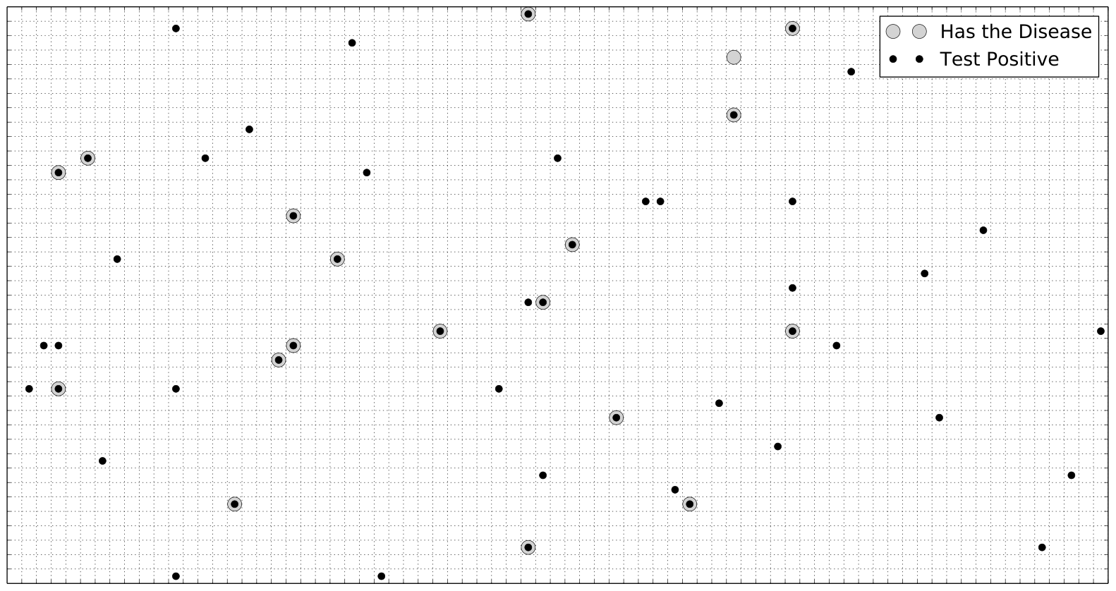
One way to see this result is to visualize it, as in Figure 5.1. Here, the numbers are a bit smaller - the disease is 1 out of 200 in a population of 3000, and the test is 99% accurate. This means about 15 sick people and about 2985 healthy people. If all of the sick people test positive, and 1% of the healthy people test positive due to the 99% accuracy, we would have 15 sick and 29 healthy people who all test positive. Even in this case, with much smaller numbers, we see that getting a positive test alone does not imply that it is likely you have the disease. It depends on the rarity of the disease (the more rare, the less likely) and the false positive rate (the number of healthy people who test positive anyway). This will vary depending on the disease and the test, but can lead to this unintuitive result, and thus can lead one to make poor medical decisions.

Function graph showing y = x*a/(x*a+(100-x)*(1-a)) on x in [0, 2] with the region between the curve and the x-axis shaded and y = 0.5. Adjustable parameter: Test accuracy (a) = 0.99. Viewing window: x from -0.14 to 2.04, y from -0.13 to 1.09. — The chance you actually have the disease given a positive test, plotted against how common the disease is. The horizontal axis is the prevalence as a PERCENTAGE of the population, so the section's second example - 1 person in 200, a test that is 99% accurate - sits at 0.5 on the axis, where the curve reads 0.33, matching the 15 sick against 29 healthy false positives the figure counts out. The dashed line is a coin flip: with a 99% test the curve only crosses it at 1% prevalence, so for anything rarer than 1 in 100 a positive result still leaves you more likely well than sick. Drag the accuracy slider up: at 99.9% the crossing moves to 0.1% prevalence, and at 99.99% to 0.01%. That is the whole content of the one-in-a-million opening - its prevalence is 0.0001 on this axis, a hundredth of a pixel from the origin, and even the 99.9% test leaves you at 0.001. Drag the accuracy down instead and watch how fast a merely good test becomes useless.

Grid of 3,000 tiny dots representing a population in which 1 in 200 people has a rare disease. Large gray circles mark the roughly 15 people who actually have the disease; black dots mark everyone who tests positive. Most large circles contain a black dot, but many black dots stand alone — false positives far outnumber the true cases. — **Figure 5.1.** Rare disease and testing. Shown is a population of 3000 where 1 in every 200 people have the disease (large circles). A test which is 99% effective is applied to everyone in the population, and the positive test results (i.e. the test says that you have the disease) are shown ask small black dots. Notice that although nearly all of those that have the disease test positive (a small black dot inside a large circle), there are many false positives (black dot in an empty square) - healthy people that test positive for the disease. Even though the test is quite good, there are many more healthy people and 1 out of 100 of them will erroneously test positive.

Consequences

This sort of disease testing has serious consequences, especially for rare diseases with tests that aren't precise. In the book “The Theory That Would Not Die: How Bayes' Rule Cracked the Enigma Code, Hunted Down Russian Submarines, and Emerged Triumphant from Two Centuries of Controversy” by Sharon McGrayne there is a discussion concerning the 2009 advice from the U.S. government task force that “most women in their forties not to have annual mammograms.” (emphasis mine) According to McGrayne,

Thus the probability that a woman who tests positive has breast cancer is only 3%. She has 97 chances out of 100 to be disease free. None of this is static. Each time more research data become available, Bayes' rule should be recalculated. As far as Bayes is concerned, universal screening for a disease that affects only 4/10 of 1% of the population may subject many healthy women to needless worry and to additional treatment which in turn can cause its own medical problems. In addition, the money spent on universal screening could potentially be used for other worthwhile projects. Thus Bayes highlights the importance of improving breast cancer screening techniques and reducing the number of false positives.¹ (emphasis mine)

Thus the proper application of probability theory allows us to separate true but unintuitive things from this which only seem true and intuitive but are in fact false.

Adapted from Statistical Inference for Everyone, by Brian Blais (Bryant University), licensed under CC BY-SA 4.0 (dual-licensed under the GNU FDL 1.2 or later; this adaptation uses the CC BY-SA grant). Changes were made; this adaptation is distributed under the same license. License: CC-BY-SA-4.0.