
3.6 Computer Examples
This section summarizes how to make histograms and scatter plots with the computer software.
Histograms
from sie import *Load a sample data set, and select only the Male data...
data=load_data('data/survey.csv')
male_data=data[data['Sex']=='Male']
select only the height data, and drop the missing data (na)...
male_height=male_data['Height'].dropna()make the histogram
hist(male_height,bins=20)
xlabel('Height [cm]')
ylabel('Number of People')
Show expected output
<matplotlib.text.Text at 0x1085728d0>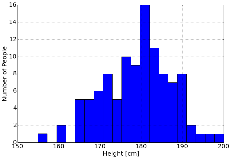
Scatter Plot
from sie import *Load a sample data set, and select only the Male data...
data=load_data('data/survey.csv')
male_data=data[data['Sex']=='Male']
select only the height and the width of writing hand data, and drop the missing data (na)...
subdata=male_data[['Height','Wr.Hnd']].dropna()
height=subdata['Height']
wr_hand=subdata['Wr.Hnd']
plot the data
plot(height,wr_hand,'o')
ylabel('Writing Hand Span [cm]')
xlabel('Height [cm]')
Show expected output
<matplotlib.text.Text at 0x1085774d0>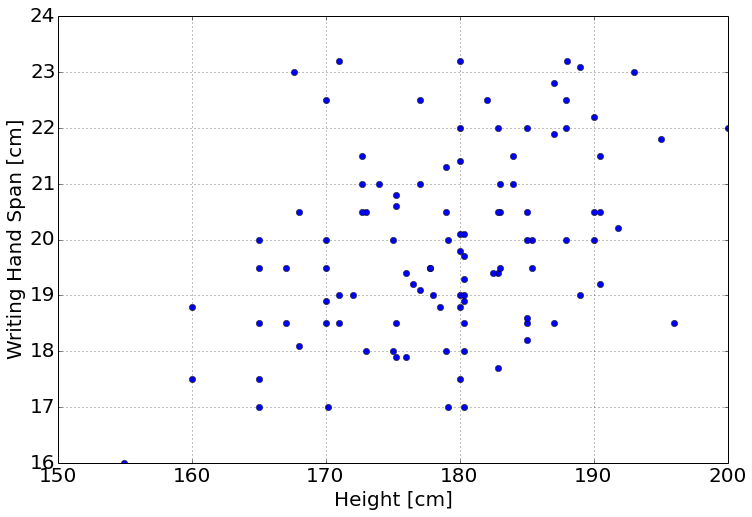
Adapted from Statistical Inference for Everyone, by Brian Blais (Bryant University), licensed under CC BY-SA 4.0 (dual-licensed under the GNU FDL 1.2 or later; this adaptation uses the CC BY-SA grant). Changes were made; this adaptation is distributed under the same license. License: CC-BY-SA-4.0.