
2.10 Computer Examples
Coin Flips
from sie import *Generate a small list of data...
data=randint(2,size=10)
print data
Show expected output
[1 0 0 1 0 0 0 1 0 0]Generate a slightly larger list of data...
data=randint(2,size=30)
print data
Show expected output
[1 1 1 0 0 0 0 1 1 1 1 0 1 1 0 1 1 0 0 1 1 1 0 1 0 0 1 1 0 0]data=randint(2,size=(2000,10))
dataShow expected output
array([[1, 0, 1, ..., 1, 0, 0],
       [1, 1, 1, ..., 0, 1, 0],
       [0, 0, 1, ..., 0, 0, 0],
       ...,
       [0, 0, 0, ..., 1, 1, 0],
       [0, 1, 0, ..., 0, 1, 1],
       [0, 1, 1, ..., 1, 0, 1]])
We have here a large collection of numbers (20000 of them!), organized in 2000 rows of 10 columns. We can sum all of the 20000 values, or we can sum across columns or across rows, depending on what we want.
sum(data) # add up all of the 1'sShow expected output
9988sum(data,axis=0) # sum up all of the columnsShow expected output
array([1011, 1010, 1001, 1051, 1001, 1008, 962, 990, 976, 978])sum(data,axis=1) # sum up all of the rowsShow expected output
array([3, 7, 3, ..., 5, 4, 6])Typically the hist command makes its own bins, which may not center on the actual count values. That's why we call countbins(N), to make bins centered on the counts.
N=sum(data,axis=1)  # number of heads in each of many flips
hist(N,countbins(10))
xlabel('Number of Heads')
ylabel('Number of Flips')
Show expected output
<matplotlib.text.Text at 0x10856e990>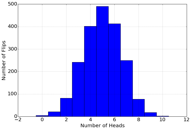
To get a probability distribution, we divide the histogram result by .
This distribution is Bernoulli's equation, or in other words, the binomial distribution.
h=array([0,1,2,3,4,5,6,7,8,9,10])

# or...

h=arange(0,11)
(recall that ** is exponentiation in Python, because the caret (^) was already used for a computer-sciency role.) The spaces in the equation below are not needed, but highlight the three parts of the binomial distribution.
from scipy.special import comb as nchoosek
p=nchoosek(10,h)* 0.5**h * 0.5**(10-h)
hist(N,countbins(10),density=True)
plot(h,p,'--o')
xlabel('Number of Heads, $h$')
ylabel('$p(h|N=10)$')Show expected output
<matplotlib.text.Text at 0x108560290>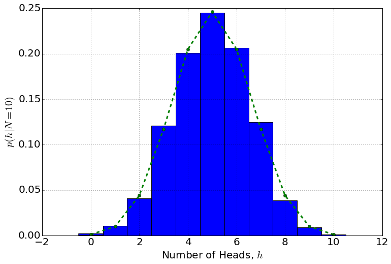
Adapted from Statistical Inference for Everyone, by Brian Blais (Bryant University), licensed under CC BY-SA 4.0 (dual-licensed under the GNU FDL 1.2 or later; this adaptation uses the CC BY-SA grant). Changes were made; this adaptation is distributed under the same license. License: CC-BY-SA-4.0.