12.3 Linear Regression

Watch demo video

We can use the variables x and y to model a linear relationship between x and y with a linear equation of the form $y = b + m x$ .

The Least-Squares method can be used to obtain the predicted y values $y ^$ as follows:

$\hat{y} = a + b x$

Where

$b = s l o p e = r \times \frac{s_{y}}{s_{x}}$ and $a = \bar{y} - b \bar{x}$

Where $s_{y}$ and $s_{x}$ are std for x and y. The following code can be used to obtain the slope and intercept.

from scipy import stats
stats.linregress(x, y)

Example: The midterm exam out of a total of 100 points, x, and final exam out of a total of 200 points, y, scores for a random sample of 11 students is listed below. Find the slope and intercept of the regression line. Test if the correlation between x and y is significant at 0.05 level of significance.

x	65	67	71	71	66	75	67	70	71	69	69
y	145	133	185	163	126	198	153	163	159	151	159

x = [65, 67, 71, 71, 66, 75, 67, 70, 71, 69, 69]
y = [145, 133, 185, 163, 126, 198, 153, 163, 159, 151, 159]
from scipy import stats
stats.linregress(x, y)

Show expected output

LinregressResult(slope=6.364142538975501, intercept=-282.5556792873051, rvalue=0.8797451071731136, pvalue=0.00035593568153235875, stderr=1.1464698617902889)

Interpretation: slope=6.364142538975501, intercept=-282.5556792873051, rvalue=0.8797451071731136 (this is Pearson correlation coefficient), pvalue=0.00035593568153235875 (this p-value is for testing the significance of the correlation coefficient), stderr=1.1464698617902889

Since the p-value is less 0.05, there is significant correlation between x and y.

slope=6.364142538975501, intercept=-282.5556792873051.

Thus, $\hat{y} = - 282.56 + 6.36 x$ is the regression line with values rounded to two decimal places.

Example: he number of hours studied, x, and test scores, y, for 10 students are listed below. Find the the correlation coefficient (r-value), estimated slope and y-intercept of the regression line and the p-value for testing the significance of correlation.

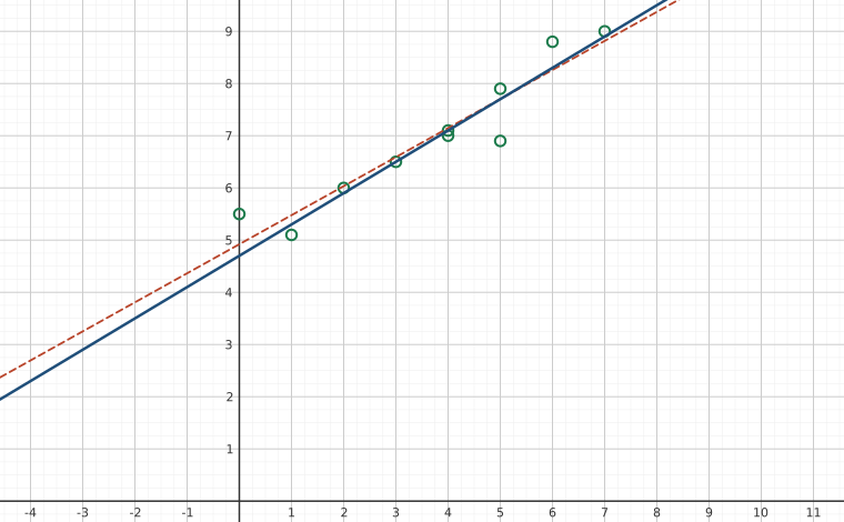
x	2	0	3	5	4	7	4	6	5	1
y	60	55	65	69	70	90	71	88	79	51

from scipy import stats

x=[2,0,3,5,4,7,4,6,5,1]
y=[60,55,65,69,70,90,71,88,79,51]

stats.linregress(x,y)

Show expected output

LinregressResult(slope=5.564625850340137, intercept=49.21088435374149, rvalue=0.9485857685252971, pvalue=2.8725087369610658e-05, stderr=0.6564713967897522)

Interpretation:

slope=5.564625850340137, intercept=49.21088435374149, r-value=0.9485857685252971, pvalue=2.8725087369610658e-05

import matplotlib.pyplot as plt
import numpy as np


x=[2,0,3,5,4,7,4,6,5,1]
y=[60,55,65,69,70,90,71,88,79,51]

x = np.array(x)
y = np.array(y)

y_hat = 5.564625850340137*x + 49.21088435374149

plt.scatter(x,y)
plt.plot(x,y_hat)

Show expected output

[<matplotlib.lines.Line2D at 0x7fa3d937f8d0>]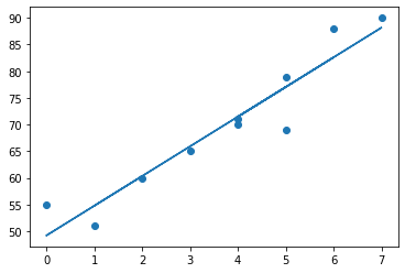

The hours-studied scatter plot with the fitted regression line ŷ = 5.56x + 49.21 drawn through the ten points.

Adapted from Python for Introductory Statistics, by Simon Aman (Truman College, City Colleges of Chicago), licensed under CC BY 4.0. Changes were made: reformatted as an accessible XYZ web edition with live in-browser code cells. License: CC-BY-4.0.