12.2 The Pearson Correlation Coefficient

The (Pearson) correlation coefficient is a measure of the strength and direction of the linear relationship between two variables.

$ρ = \frac{c o v (x, y)}{σ_{x} σ_{y}}$ for population correlation coefficient

$r = \frac{c o v (x, y)}{s_{x} s_{y}}$ or $r = \frac{n Σ x y - Σ x Σ y}{\sqrt{n Σ x^{2} - (Σ x)^{2}} \sqrt{n Σ y^{2} - (Σ y)^{2}}}$ for sample correlation coefficient

Where $ρ$ and $r$ are the population and sample Pearson correlation coefficients respectively. $c o v (x, y)$ is the covariance of the two variables.

The value of r is between -1 and 1 and it is unitless. That is, it is not affected by the unit of measurements of both variables.

if $r$ or $ρ$ is close to +1, we conclude strong positive relationship
If $r$ or $ρ$ is close to -1, we conclude strong negative relationship
If $r$ or $ρ$ is close to zero, we conclude weak or no relationship

To compute the correlation coefficient, you can use of the following two options.

from scipy import stats
stats.linregress(x, y)  # rvalue the 3rd from the output

import numpy as np
x = [x1,x2,...]
y = [y1,y2,...]
np.corrcoef(x,y)

returns a matrix form of correlations between x and x, x and y, y and x, y and y

Example: The midterm exam out of a total of 100 points, x, and final exam out of a total of 200 points, y, scores for a random sample of 11 students is listed below. Find the correlation coefficient and draw a scatter plot.

x	65	67	71	71	66	75	67	70	71	69	69
y	145	133	185	163	126	198	153	163	159	151	159

Watch demo video 1 Scatter Plot

Watch demo video 2 Correlation Coefficient

# Pearson Correlation Coefficient
import numpy as np
x = [65, 67, 71, 71, 66, 75, 67, 70, 71, 69, 69]
y = [145, 133, 185, 163, 126, 198, 153, 163, 159, 151, 159]
np.corrcoef(x,y)

Show expected output

array([[1.        , 0.87974511],
       [0.87974511, 1.        ]])

Interpretation: Because r=0.879745 is positive and close to one, we can conclude that there is a strong and direct relationship between x midterm scores and y final exam scores.

Note: The correlation coefficient between x and x is 1. Similarly between y and y is 1.

x = [65, 67, 71, 71, 66, 75, 67, 70, 71, 69, 69]
y = [145, 133, 185, 163, 126, 198, 153, 163, 159, 151, 159]

from scipy import stats
stats.linregress(x, y)

Show expected output

LinregressResult(slope=6.364142538975501, intercept=-282.5556792873051, rvalue=0.8797451071731136, pvalue=0.00035593568153235875, stderr=1.1464698617902889)

Interpretation: for now we only need the third output rvalue=0.8797451071731136

# scatterplot
import matplotlib.pyplot as plt
x = [65, 67, 71, 71, 66, 75, 67, 70, 71, 69, 69]
y = [145, 133, 185, 163, 126, 198, 153, 163, 159, 151, 159]
plt.scatter(x, y)

Show expected output

<matplotlib.collections.PathCollection at 0x7f9c4241aa10>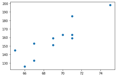

Scatter plot of the height data x (65 to 75 inches) against weight y (126 to 198 pounds): eleven points trending clearly upward, consistent with the printed r ≈ 0.88.

There is a positive or direct relationship.

Example: The number of hours studied, x, and test scores, y, for 10 students are listed below. Find the correlation coefficient and display the scatter plot.

x	2	0	3	5	4	7	4	6	5	1
y	60	55	65	69	70	90	71	88	79	51

import numpy as np

x=[2,0,3,5,4,7,4,6,5,1]
y=[60,55,65,69,70,90,71,88,79,51]

np.corrcoef(x,y)

Show expected output

array([[1.        , 0.94858577],
       [0.94858577, 1.        ]])

import matplotlib.pyplot as plt

x=[2,0,3,5,4,7,4,6,5,1]
y=[60,55,65,69,70,90,71,88,79,51]

plt.scatter(x,y)

Show expected output

<matplotlib.collections.PathCollection at 0x7fa3da036dd0>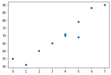

Scatter plot of hours studied (0 to 7) against test scores (51 to 90) for the ten students: the points rise to the right.

Adapted from Python for Introductory Statistics, by Simon Aman (Truman College, City Colleges of Chicago), licensed under CC BY 4.0. Changes were made: reformatted as an accessible XYZ web edition with live in-browser code cells. License: CC-BY-4.0.