14.5 Inferential Statistics for b and r

This section shows how to conduct significance tests and compute confidence intervals for the regression slope and Pearson's correlation. As you will see, if the regression slope is significantly different from zero, then the correlation coefficient is also significantly different from zero.

Assumptions

Although no assumptions were needed to determine the best-fitting straight line, assumptions are made in the calculation of inferential statistics. Naturally, these assumptions refer to the population, not the sample.

Linearity: The relationship between the two variables is linear.
Homoscedasticity: The variance around the regression line is the same for all values of X. A clear violation of this assumption is shown in Figure 1. Notice that the predictions for students with high high-school GPAs are very good, whereas the predictions for students with low high-school GPAs are not very good. In other words, the points for students with high high-school GPAs are close to the regression line, whereas the points for low high-school GPA students are not.
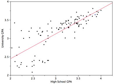
Figure 1. University GPA as a function of High School GPA.
The errors of prediction are distributed normally. This means that the deviations from the regression line are normally distributed. It does not mean that X or Y is normally distributed.

Significance Test for the Slope (b)

Recall the general formula for a t test:

$t = \frac{statistic - hypothesized value}{estimated standard error of the statistic}$

As applied here, the statistic is the sample value of the slope (b) and the hypothesized value is 0. The number of degrees of freedom for this test is:

df = N-2

where N is the number of pairs of scores.

The estimated standard error of b is computed using the following formula:

$s_{b} = \frac{s_{est}}{\sqrt{S S X}}$

where s_b is the estimated standard error of b, s_est is the standard error of the estimate, and SSX is the sum of squared deviations of X from the mean of X. SSX is calculated as

$S S X = \sum (X - M_{X})^{2}$

where M_x is the mean of X. As shown previously, the standard error of the estimate can be calculated as

$s_{est} = \sqrt{\frac{(1 - r^{2}) S S Y}{N - 2}}$

These formulas are illustrated with the data shown in Table 1. These data are reproduced from the introductory section. The column X has the values of the predictor variable and the column Y has the values of the criterion variable. The third column, x, contains the differences between the values of column X and the mean of X. The fourth column, x², is the square of the x column. The fifth column, y, contains the differences between the values of column Y and the mean of Y. The last column, y², is simply square of the y column.

Table 1. Example data.

	X	Y	x	x²	y	y²
	1.00	1.00	-2.00	4	-1.06	1.1236
	2.00	2.00	-1.00	1	-0.06	0.0036
	3.00	1.30	0.00	0	-0.76	0.5776
	4.00	3.75	1.00	1	1.69	2.8561
	5.00	2.25	2.00	4	0.19	0.0361
Sum	15.00	10.30	0.00	10.00	0.00	4.5970

The computation of the standard error of the estimate (s_est) for these data is shown in the section on the standard error of the estimate. It is equal to 0.964.

s_est = 0.964

SSX is the sum of squared deviations from the mean of X. It is, therefore, equal to the sum of the x² column and is equal to 10.

SSX = 10.00

We now have all the information to compute the standard error of b:

$s_{b} = \frac{0.964}{\sqrt{10}} = 0.305$

As shown previously, the slope (b) is 0.425. Therefore,

$t = \frac{0.425}{0.305} = 1.39$

df = N-2 = 5-2 = 3.

The p value for a two-tailed t test is 0.26. Therefore, the slope is not significantly different from 0.

Confidence Interval for the Slope

The method for computing a confidence interval for the population slope is very similar to methods for computing other confidence intervals. For the 95% confidence interval, the formula is:

lower limit: b - (t_.95)(s_b)
upper limit: b + (t_.95)(s_b)

where t_.95 is the value of t to use for the 95% confidence interval.

The values of t to be used in a confidence interval can be looked up in a table of the t distribution. A small version of such a table is shown in Table 2. The first column, df, stands for degrees of freedom.

Table 2. Abbreviated t table.

df	0.95	0.99
2	4.303	9.925
3	3.182	5.841
4	2.776	4.604
5	2.571	4.032
8	2.306	3.355
10	2.228	3.169
20	2.086	2.845
50	2.009	2.678
100	1.984	2.626

You can also use the "inverse t distribution" calculator to find the t values to use in a confidence interval.

Applying these formulas to the example data,

lower limit: 0.425 - (3.182)(0.305) = -0.55
upper limit: 0.425 + (3.182)(0.305) = 1.40

Significance Test for the Correlation

The formula for a significance test of Pearson's correlation is shown below:

$t = \frac{r \sqrt{N - 2}}{\sqrt{1 - r^{2}}}$

where N is the number of pairs of scores. For the example data,

$t = \frac{0.627 \sqrt{5 - 2}}{\sqrt{1 - {0.627}^{2}}} = 1.39$

Notice that this is the same t value obtained in the t test of b. As in that test, the degrees of freedom is N - 2 = 5 -2 = 3.

Adapted from Online Statistics Education: A Multimedia Course of Study (onlinestatbook.com), Project Leader: David M. Lane, Rice University. Developed with NSF support. The original work is in the public domain; it is cited here at the authors' request. Changes were made: reformatted as an accessible XYZ web edition with native MathML. License: Public-Domain.