14.4 Standard Error of the Estimate

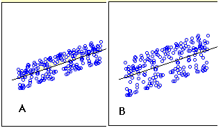
Figure 1 shows two regression examples. You can see that in Graph A, the points are closer to the line than they are in Graph B. Therefore, the predictions in Graph A are more accurate than in Graph B.

Two scatter plots labeled A and B, each with the same rising regression line through a cloud of circles. In A the points lie in a tight band about the line; in B the same number of points scatter much more widely around it. The predictions in A are more accurate — A has the smaller standard error of the estimate. — Figure 1. Regressions differing in accuracy of prediction.

The standard error of the estimate is a measure of the accuracy of predictions. Recall that the regression line is the line that minimizes the sum of squared deviations of prediction (also called the sum of squares error). The standard error of the estimate is closely related to this quantity and is defined below:

$σ_{est} = \sqrt{\frac{\sum (Y - Y^{'})^{2}}{N}}$

where σ_est is the standard error of the estimate, Y is an actual score, Y' is a predicted score, and N is the number of pairs of scores. The numerator is the sum of squared differences between the actual scores and the predicted scores.

Note the similarity of the formula for σ_est to the formula for σ. It turns out that σest is the standard deviation of the errors of prediction (each Y - Y' is an error of prediction).

Assume the data in Table 1 are the data from a population of five X, Y pairs.

Table 1. Example data.

	X	Y	Y'	Y-Y'	(Y-Y')²
	1.00	1.00	1.210	-0.210	0.044
	2.00	2.00	1.635	0.365	0.133
	3.00	1.30	2.060	-0.760	0.578
	4.00	3.75	2.485	1.265	1.600
	5.00	2.25	2.910	-0.660	0.436
Sum	15.00	10.30	10.30	0.000	2.791

The last column shows that the sum of the squared errors of prediction is 2.791. Therefore, the standard error of the estimate is

$σ_{est} = \sqrt{\frac{2.791}{5}} = 0.747$

There is a version of the formula for the standard error in terms of Pearson's correlation:

$σ_{est} = \sqrt{\frac{(1 - ρ^{2}) S S Y}{N}}$

where ρ is the population value of Pearson's correlation and SSY is

$S S Y = \sum (Y - μ_{Y})^{2}$

For the data in Table 1, μ_y = 2.06, SSY = 4.597 and ρ= 0.6268. Therefore,

$σ_{est} = \sqrt{\frac{(1 - {0.6268}^{2}) (4.597)}{5}} = \sqrt{\frac{2.791}{5}} = 0.747$

which is the same value computed previously.

Similar formulas are used when the standard error of the estimate is computed from a sample rather than a population. The only difference is that the denominator is N-2 rather than N. The reason N-2 is used rather than N-1 is that two parameters (the slope and the intercept) were estimated in order to estimate the sum of squares. Formulas for a sample comparable to the ones for a population are shown below.

$s_{est} = \sqrt{\frac{\sum (Y - Y^{'})^{2}}{N - 2}}$

$s_{est} = \sqrt{\frac{2.791}{3}} = 0.964$

$s_{est} = \sqrt{\frac{(1 - r^{2}) S S Y}{N - 2}}$

x=c(1,2,3,4,5) y= c(1,2,1.3,3.75,2.25) summary(lm(y~x)) Call: lm(formula = y ~ x) Residuals: 1 2 3 4 5 -0.210 0.365 -0.760 1.265 -0.660 Coefficients: Estimate Std. Error t value Pr(>|t|) (Intercept) 0.785 1.012 0.776 0.494 x 0.425 0.305 1.393 0.258 Residual standard error: 0.9645 on 3 degrees of freedom Multiple R-squared: 0.3929, Adjusted R-squared: 0.1906 F-statistic: 1.942 on 1 and 3 DF, p-value: 0.2578

Adapted from Online Statistics Education: A Multimedia Course of Study (onlinestatbook.com), Project Leader: David M. Lane, Rice University. Developed with NSF support. The original work is in the public domain; it is cited here at the authors' request. Changes were made: reformatted as an accessible XYZ web edition with native MathML. License: Public-Domain.