In our basic exponential growth scenario, we had a recursive equation of the form
In a confined environment, however, the growth rate may not remain constant. In a lake, for example, there is some maximum sustainable population of fish, also called a carrying capacity.
For our fish, the carrying capacity is the largest population that the resources in the lake can sustain. If the population in the lake is far below the carrying capacity, then we would expect the population to grow essentially exponentially. However, as the population approaches the carrying capacity, there will be a scarcity of food and space available, and the growth rate will decrease. If the population exceeds the carrying capacity, there won’t be enough resources to sustain all the fish and there will be a negative growth rate, causing the population to decrease back to the carrying capacity.
If the carrying capacity was 5000, the growth rate might vary something like that in the graph shown. Note that this is a linear equation with intercept at and slope , so we could write an equation for this adjusted growth rate as:
Substituting this in to our original exponential growth model for gives
Unlike linear and exponential growth, logistic growth behaves differently if the populations grow steadily throughout the year or if they have one breeding time per year. The recursive formula provided above models generational growth, where there is one breeding time per year (or, at least a finite number); there is no explicit formula for this type of logistic growth.
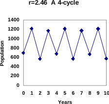
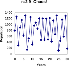
Taking this even further, we get more and more extreme behaviors as the growth rate increases higher. It is possible to get stable 4-cycles, 8-cycles, and higher. Quickly, though, the behavior approaches chaos (remember the movie Jurassic Park?).
Adapted from Math in Society by David Lippman, hosted on LibreTexts (math.libretexts.org) and licensed under CC BY-SA 3.0. Changes were made. License: CC-BY-SA-3.0.
These eBooks are a prerelease and are not yet certified conformant with WCAG 2.1 AA or any other accessibility standard. Every page is built against an automated accessibility gate, and our target for the published editions is WCAG 2.2 Level AA. If something is unusable, please tell us.

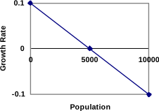 If the carrying capacity was 5000, the growth rate might vary something like that in the graph shown. Note that this is a linear equation with intercept at and slope , so we could write an equation for this adjusted growth rate as: