1.3 Harvesting and Bifurcation

Take last section's pond and start fishing it. If boats remove a fixed quantity per unit time — a quota, not a percentage — the model gains a constant subtraction:

$\frac{dP}{dt} = 2P\left(1 - \frac{P}{8}\right) - a,$

where $a \ge 0$ is the harvest rate. The question a fishery manager actually asks is not "what is $P(t)$ ?" but "how large can $a$ be before the pond collapses?" That question is about equilibria, and equilibria can be found without solving anything: set the right-hand side to zero.

Expanding, $2P - P^2/4 - a = 0$ , or $P^2 - 8P + 4a = 0$ , whose roots are

$P_{\pm} = 4 \pm \sqrt{16 - 4a}.$

Everything interesting is in that square root. For $a < 4$ there are two equilibria, one above the midpoint $4$ and one below. At $a = 4$ the root vanishes and the two merge into a single equilibrium at $P = 4$ . For $a > 4$ there is no real root at all: no equilibrium exists, $dP/dt$ is negative for every population, and the fishery drives itself to zero no matter how healthy it started.

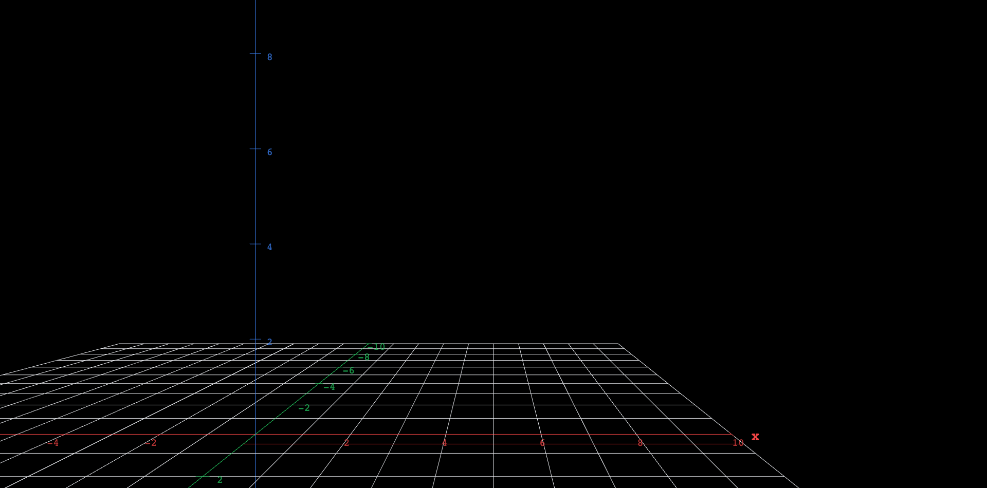
The figure below shows the two equilibrium levels as horizontal lines whose heights you control with the harvest slider.

-\left(-8 \cdot P + 4 \cdot a + P^{2}\right) - 4 \cdot \left(2 \cdot P - a - \frac{1}{4} \cdot P^{2}\right)

The rearrangement, verified ✓ Computed · mojocas 0.1.0 ✓ Agrees with the text

The word "or" in the paragraph above is doing real work: it asserts that $2P - P^2/4 - a = 0$ and $P^2 - 8P + 4a = 0$ have the same solutions. They do — the second is the first multiplied by $-4$ — and multiplying an equation by a nonzero constant is exactly the operation that preserves a solution set. This card subtracts one side from $-4$ times the other and certifies the difference is identically zero, so every equilibrium claim that follows rests on the polynomial the section actually solves.

4 + 2 \cdot \sqrt{4 - a},\; 4 - 2 \cdot \sqrt{4 - a}

The closed form, for every harvest rate at once ✓ Computed · mojocas 0.1.0 ✓ Agrees with the text

The formula itself, certified — not at one rate, but as an identity in $a$ .

It is worth knowing what had to happen for this card to exist. The engine solves the quadratic to $4 \pm 2\sqrt{4-a}$ ; the section writes $4 \pm \sqrt{16-4a}$ . Those are the same number — $16 - 4a = 4(4-a)$ and $\sqrt{4} = 2$ — but a computer algebra system will not treat two radicals as equal just because a human can factor one into the other. Until the engine learned to pull the perfect-square part out of a radicand's content, the two spellings were simply different atoms, and this section's own closed form was the one claim in the chapter that could not be checked.

Note what the certificate does not assume. Nothing here requires $a \le 4$ : the sign of $4 - a$ stays inside the radical, so the identity holds as written for every $a$ , real or otherwise. That the root turns imaginary past $a = 4$ is the mathematics the section is about — the bifurcation — not a caveat on the algebra.

Two horizontal lines in the plane: a solid green line (the stable equilibrium population) and a dashed red line below it (the unstable threshold). Dragging the harvest slider a from 0 toward 4 pulls the green line down from 8 and the red line up from 0 until the two meet at height 4 exactly when a reaches 4, where both equilibria disappear together. — Equilibria of the harvested logistic model. The solid green line is $P_+ = 4 + \sqrt{16 - 4a}$ and the dashed red line is $P_- = 4 - \sqrt{16 - 4a}$ . Dragging the harvest rate $a$ toward $4$ squeezes the two together until they collide and disappear.

Explore

Observe. Start with $a = 0$ (no fishing). Where do the two lines sit? Confirm they are the equilibria $0$ and $8$ you already know from the unharvested logistic equation.
Predict. As $a$ increases, one line must move up and the other down. Which is which, and why? Write down your reasoning from the formula before dragging.
Verify. Drag $a$ slowly from $0$ to $3$ . Note the gap between the lines at $a = 1$ , at $a = 2$ , and at $a = 3$ . Is the gap shrinking at a steady rate, or is it collapsing faster near the end?
Observe. Push $a$ to $3.9$ , then to $3.99$ . Both lines are now nearly at height $4$ . The square root is what makes the last stretch so abrupt — the gap is $2\sqrt{16 - 4a}$ , so what happens to the rate of collapse as $a \to 4$ ?
Predict, then reason. The green line is stable and the red one unstable. If the pond is sitting comfortably at $P_+$ with $a = 3.9$ and a storm knocks the population down by $1$ , does it recover? Now suppose the harvest is raised to $a = 4.1$ instead: what happens to a pond sitting at $P = 4$ ?

Connect

A bifurcation is a qualitative change in the set of equilibria caused by a smooth change in a parameter. Here, nudging $a$ through the critical value $4$ does not merely move the equilibria — it destroys them. Two equilibria of opposite stability approach each other, merge, and annihilate; this pattern is common enough to have a name, the saddle-node (or fold) bifurcation, and it is the mathematical signature of a system that fails suddenly rather than gradually.

The management lesson is sharper than the equations look. Just below the critical rate, the pond still has a stable equilibrium, so the fishery appears to be working — but the unstable equilibrium $P_-$ has crept up close underneath it, which means the margin for error has nearly vanished. A bad season that pushes the population below $P_-$ sends it to extinction even though the harvest rate never changed. Systems near a saddle-node bifurcation look healthy right up until they do not, and the shrinking gap you watched in step 3 is exactly the shrinking margin.

6,\; 2

The two equilibria at a = 3 ✓ Computed · mojocas 0.1.0 ✓ Agrees with the text

The worked example's quota, solved. Both equilibria are exact integers, so the safety margin $P_+ - P_- = 4$ is exact too — the number a manager would actually plan against.

8,\; 0

No fishing returns the pond you started with ✓ Computed · mojocas 0.1.0 ✓ Agrees with the text

Explore step 1 asks you to confirm that setting $a = 0$ recovers the unharvested logistic equilibria. Set $a = 0$ in $P^2 - 8P + 4a = 0$ and the roots are $0$ and $8$ , exactly the pair from the previous section. The harvest term is the only thing that moved them.

Euler's Method

Everything above was equilibrium reasoning, which needs no solution formula — fortunate, because the harvested logistic equation's solutions are unpleasant to write down and most equations have none at all. The general escape is numerical. Euler's method takes the equation's own instruction, $y' = f(t, y)$ , and treats it as a recipe for one small step: from the point you are standing on, set off along the slope the equation gives there, walk for a time $h$ , and repeat. Each step is exact only at its start, so the polygon it traces drifts away from the true solution — and the size of that drift is the whole question.

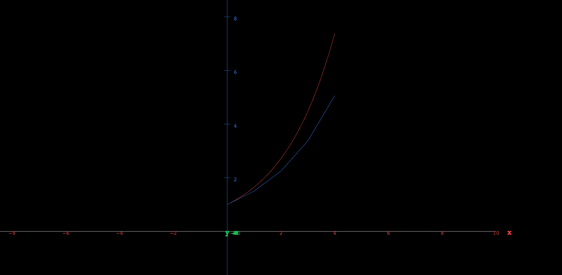
To see the drift clearly, run the method on an equation we can solve, $y' = by$ with $y(0) = 1$ , whose true solution is $y = e^{bt}$ .

A smooth red exponential curve rises from height 1 at the left edge, and a blue polygonal path starts at the same point and chases it: straight segments that each set off along the curve's slope, then fall behind as the curve bends upward, so the polygon sags visibly below the curve and the gap widens to the right. The slider h sets the length of each straight segment — at large h the polygon is a few long chords far below the curve, and as h shrinks the corners multiply and the polygon hugs the curve until the two are hard to tell apart. The slider b steepens both together. — Euler's method on $y' = by$ from $y(0) = 1$ . The smooth red curve is the true solution $e^{bt}$ ; the blue polygon is the Euler approximation with step size $h$ . Each blue segment leaves along the slope the equation gives at its left endpoint, so the polygon consistently falls below a curve that is bending upward.

Observe. Start at $h = 1$ , $b = 0.5$ . Count the straight segments in the blue path and find the corners between them. At which end of each segment does the polygon agree with the red curve?
Predict. The curve bends upward everywhere. Will the polygon sit above it or below it? Commit to an answer and give a one-sentence reason before dragging anything.
Verify. Read the vertical gap between the two paths at the right edge with $h = 1$ , then halve the step to $h = 0.5$ . Roughly what fraction of the error survives? Halve it again to $h = 0.25$ and check whether that fraction repeats.
Observe. Push $h$ to $2$ . The polygon is now a couple of long chords far below the curve. Is the method wrong here, or just coarse — and how would you tell the difference from the picture alone?
Predict, then verify. Raise $b$ to $0.9$ with $h$ fixed. Does the error at the right edge grow, shrink, or stay put? Explain from the fact that a larger $b$ makes the true curve bend harder.

Halving the step roughly halves the error: Euler's method is first order. That is why it is the first method taught and rarely the one used — the methods behind the trajectory curves later in this book take the same idea and sample the slope more than once per step, buying a far better error for the same amount of walking.

An original work of XYZ Homework, built around interactive XYZ 3D figures, following the standard first-course sequence (first-order equations through systems and the phase plane). Distinct from the LibreTexts-sourced Differential Equations for Engineers (Lebl) edition, which has its own attribution. License: CC-BY-NC-SA-4.0.