1.1 Solution Families

The shortest differential equation with something to say is

$\frac{d y}{d t} = k y .$

In words: the rate of change of $y$ is proportional to $y$ itself. Money earning continuous interest obeys it, a bacterial culture with unlimited food obeys it, a radioactive sample obeys it with $k$ negative. The equation does not mention any particular starting amount — and that is the point. A differential equation constrains the shape of a solution, not its starting place, so it is satisfied not by one function but by a whole family of them:

$y (t) = a e^{k t},$

one member for every choice of the constant $a$ . Substitute back to check: the derivative of $a e^{k t}$ is $k \cdot a e^{k t}$ , which is exactly $k$ times the function. The constant $a$ is not decoration; it is the answer to a question the differential equation never asked, namely where does the solution start? Setting $t equals 0$ gives $y open parenthesis 0 close parenthesis equals a$ .

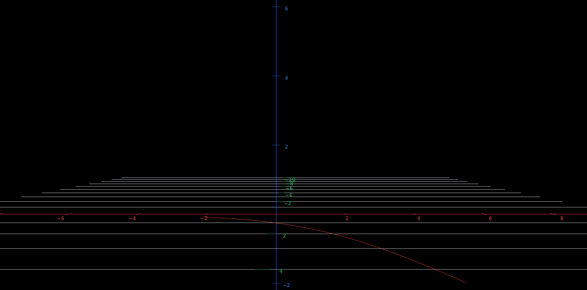
The figure below puts the whole family under your hands. The slider $a$ is the initial value $y open parenthesis 0 close parenthesis$ and the slider $b$ plays the role of the rate constant $k$ . Behind the curve is the equation's own instruction drawn everywhere at once: at each point of the plane a short segment with slope $b y$ , the slope field. The curve never leaves it — wherever the curve goes, it runs tangent to the segment it is passing.

A single red exponential curve drawn through a grid of short gray slope marks, one mark at every point of the plane, each tilted to the slope the equation y' = by assigns there: flat along the horizontal axis, steeper with height, and reversed below the axis. The curve stays tangent to every mark it crosses. The slider a slides the curve up or down through its starting value, flipping it below the axis when a is negative, where it threads the same field mirror-fashion; the slider b re-tilts the whole field and bends the curve with it, from steep growth through flat to rapid decay. — The exponential family $y = a e^{b t}$ threading the slope field of $y^{'} = b y$ . The slider $a$ sets the starting value $y open parenthesis 0 close parenthesis$ ; the slider $b$ sets the growth rate and re-tilts the whole field. Every curve these two dials can produce is a solution, and each one stays tangent to the segments it crosses.

Explore

Observe. Set $b equals 0.5$ and sweep $a$ from $3$ down through $0$ to $minus 3$ . Every curve in the sweep passes through the point $open parenthesis 0, a close parenthesis$ . What single point does the entire family have in common when $a equals 0$ ?
Predict. With $a equals 2$ fixed, what will happen to the curve as you drag $b$ from $0.5$ down through $0$ to $minus 1$ ? Sketch your guess for all three regimes before touching the slider.
Verify. Now drag $b$ . At $b equals 0$ the equation reads $y prime equals 0$ — which functions satisfy that, and is the flat line you see one of them?
Observe. Make the curve decay: $a equals 3$ , $b = - 1$ . Read off roughly where the curve has dropped to half its starting height. Then set $b = - 2$ and read the half-height time again. How did doubling the decay rate change the half-life?
Predict, then verify. Can you find slider settings that make the curve pass through the point $open parenthesis 1, 2 close parenthesis$ ? There are many — find two visibly different ones, and explain why the initial value problem $y open parenthesis 0 close parenthesis equals 2$ has only one.

Connect

An initial value problem bundles a differential equation with a starting fact: $y^{'} = k y$ together with $y open parenthesis 0 close parenthesis equals y sub 0$ . The equation supplies the family $y = a e^{k t}$ ; the initial condition picks the member with $a equals y sub 0$ ; and that member is the only one. This one-condition-one-solution pattern is the normal situation for first-order equations, and it is why the sliders in the figure feel like coordinates: the pair $(a, b)$ is a complete address for a curve. Exploration step 5 shows the flip side — a point away from $t equals 0$ does not pin down a curve unless the rate is also known, which is why the problem statement must say which equation and which starting value.

An original work of XYZ Homework, built around interactive XYZ 3D figures, following the standard first-course sequence (first-order equations through systems and the phase plane). Distinct from the LibreTexts-sourced Differential Equations for Engineers (Lebl) edition, which has its own attribution. License: CC-BY-NC-SA-4.0.