
1.2 The Logistic Equation
Exponential growth cannot last. A population that doubles every hour eventually runs out of food, space, or patience, and a model that ignores this fact answers questions about the far future with nonsense. The classical fix is to make the per-capita growth rate fall as the population rises. With carrying capacity (in whatever units the habitat supports), the logistic equation is
Read it before solving it. When is small the factor is close to and the equation is nearly — exponential growth. When is near the factor is near and growth stalls. Between them, the growth rate is largest at , halfway up. And there are two population levels where nothing changes at all: and , the equilibria, where the right-hand side vanishes and a population that starts there stays there forever.
The equation can be solved in closed form, and the solutions are
where the constant encodes the starting value: , so large means a small starting population and near zero means starting almost at capacity.
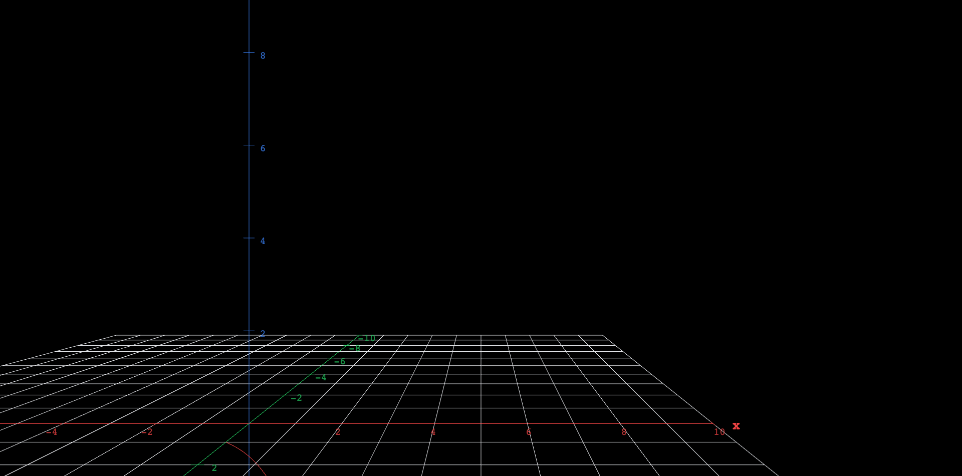 Explore in 3D (opens in a new tab)
Explore
- Observe. Set , , so . The curve is S-shaped: slow, then fast, then slow. At roughly what height is the curve steepest? Compare with the halfway level .
- Predict. If you increase to , the starting population drops to about . Will the curve still reach toward the dashed line at , or level off lower? Decide, then drag the slider.
- Verify. With any settings, zoom your attention to the right edge of the window. Does the red curve ever touch or cross the dashed line at ? Explain from the equation why it cannot: what would be at the moment of touching?
- Observe. Drag down to , so the population starts near , close to capacity. The S-shape disappears. Which part of the S did this starting value skip?
- Predict, then verify. The equilibrium is also a solution. Judging from the curves with large , does a tiny population move toward or away from it? What does that say about the stability of the extinction equilibrium?
Connect
The two dashed lines behave differently, and the difference is the most important qualitative fact about the model. Solutions that start just above flee from it: is unstable, an equilibrium in the sense of a pencil balanced on its tip. Solutions from every positive starting value climb or descend toward and flatten against it: is stable, an equilibrium like a marble at the bottom of a bowl. You verified both facts with sliders, but they were readable from the equation alone — the sign of is positive for and negative for , so arrows on a vertical -axis point away from and toward . That sign analysis, not the closed formula, is what generalizes to equations nobody can solve.
The Slope Field
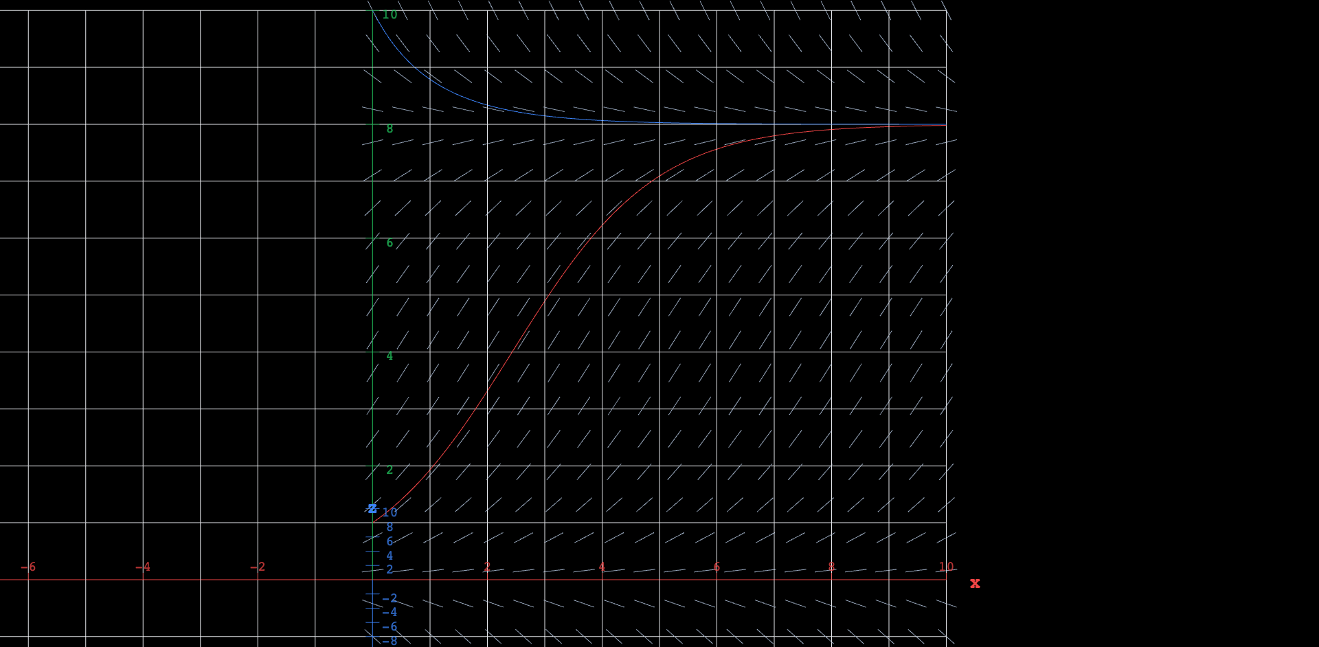
Everything above began by solving the equation. The picture below never does. A slope field draws, at every point of the plane, a short segment whose slope is — the equation's instruction at that point, available without any solution formula. A solution curve is then simply a curve that stays tangent to the segments it passes through, and the two equilibria appear as horizontal rivers the flow converges to or splits away from.
 Explore in 3D (opens in a new tab)
- Observe. Look only at the segments, ignoring the curves. Along the dashed line every segment is flat, and the same is true along . What does a flat segment say about there, and why does that make those two levels equilibria?
- Predict. Put a fingertip anywhere in the band and follow the tilts to the right. Do you end up at , at , or somewhere else? Now start above and do the same.
- Verify. The red curve starts at and the blue at . Check that each is tangent to every segment it crosses, and that they approach the line from opposite sides without touching it.
- Observe. Where in the field are the segments steepest? Compare with your answer from the first Explore list — the halfway level — and with the fact that the red curve is steepest exactly where it crosses that level.
- Predict, then verify. Drag up toward . Does the shape of the field change, or only the steepness of its segments? What does that say about which features of this model depend on and which do not?
The equilibria are exactly the levels where the field goes flat, so they can be found by setting the right-hand side to zero and solving — no solution formula involved.
Differentiating with respect to gives , and the growth rate peaks where that vanishes. The CAS solves it here: the fastest growth happens at , halfway to capacity — which is why the red curve is steepest as it crosses the middle of the band, and why the S-shape has its bend exactly there.
The certificate carries one declared hypothesis: . That is not a technicality the engine is being fussy about — if were zero the equation would hold at every population, there would be no growth to maximize, and "" would be a wrong answer dressed as a complete one. The section fixed as the growth rate in its first paragraph, so the hypothesis is the model's own; the engine simply refuses to use it without being told, and the check runs through its full case analysis rather than the generic shortcut.
An original work of XYZ Homework, built around interactive XYZ 3D figures, following the standard first-course sequence (first-order equations through systems and the phase plane). Distinct from the LibreTexts-sourced Differential Equations for Engineers (Lebl) edition, which has its own attribution. License: CC-BY-NC-SA-4.0.