A.6 Determinant

For square matrices we define a useful quantity called the determinant. Define the determinant of a $1 times 1$ matrix as the value of its only entry

$det open parenthesis [ a ] close parenthesis equals def a.$

For a

2 times 2

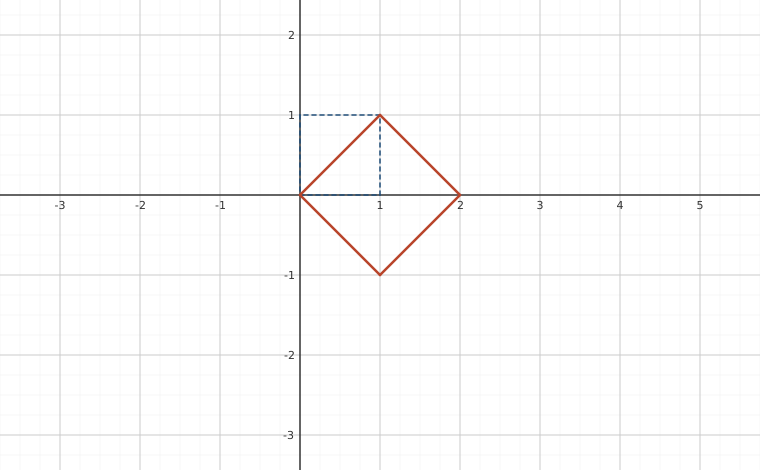
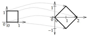
matrix, define

$det ([\begin{matrix} a & b \\ c & d \end{matrix}]) \overset{def}{=} a d - b c .$

Before defining the determinant for larger matrices, we note the meaning of the determinant. An

n \times n

matrix gives a mapping of the

n

-dimensional euclidean space

ℝ^{n}

to itself. So a

2 times 2

matrix

A

is a mapping of the plane to itself. The determinant of

A

is the factor by which the area of objects changes. If we take the unit square (square of side 1) in the plane, then

A

takes the square to a parallelogram of area

| det open parenthesis A close parenthesis |

. The sign of

det (A)

denotes a change of orientation (negative if the axes get flipped). For example, let

$A = [\begin{matrix} 1 & 1 \\ - 1 & 1 \end{matrix}] .$

Then

det (A) = 1 + 1 = 2

. Let us see where

A

sends the unit square—the square with vertices

open parenthesis 0, 0 close parenthesis

open parenthesis 1, 0 close parenthesis

open parenthesis 0, 1 close parenthesis

, and

open parenthesis 1, 1 close parenthesis

. The point

open parenthesis 0, 0 close parenthesis

gets sent to

open parenthesis 0, 0 close parenthesis

$[\begin{matrix} 1 & 1 \\ - 1 & 1 \end{matrix}] [\begin{matrix} 1 \\ 0 \end{matrix}] = [\begin{matrix} 1 \\ - 1 \end{matrix}], [\begin{matrix} 1 & 1 \\ - 1 & 1 \end{matrix}] [\begin{matrix} 0 \\ 1 \end{matrix}] = [\begin{matrix} 1 \\ 1 \end{matrix}], [\begin{matrix} 1 & 1 \\ - 1 & 1 \end{matrix}] [\begin{matrix} 1 \\ 1 \end{matrix}] = [\begin{matrix} 2 \\ 0 \end{matrix}] .$

The image of the square is another square with vertices

open parenthesis 0, 0 close parenthesis

open parenthesis 1, minus 1 close parenthesis

open parenthesis 1, 1 close parenthesis

, and

open parenthesis 2, 0 close parenthesis

. The image square has a side of length

the square root of 2

, and it is therefore of area

2

. See Figure

1

Function graph showing the parametric curve (t, 0) for t in [0, 1], the parametric curve (1, t) for t in [0, 1], the parametric curve (1-t, 1) for t in [0, 1], the parametric curve (0, 1-t) for t in [0, 1], the parametric curve (t, -t) for t in [0, 1], the parametric curve (1+t, -1+d*t) for t in [0, 1], the parametric curve (2-t, (d-1)+t) for t in [0, 1] and the parametric curve (1-t, d-d*t) for t in [0, 1]. Adjustable parameter: Lower-right entry d (d) = 1. Viewing window: x from -3.75 to 5.75, y from -3.44 to 2.44. — A = [1 1; −1 d] applied to the unit square (dashed blue) — at the default d = 1 this is the section's own example, det A = 2, and the image parallelogram (orange) has area |det A| = |d + 1|. Drag d down through −1 to collapse the parallelogram onto a single segment (area 0, the two columns identical, so A is not invertible), then keep going to see the orientation flip that the sign of det A records.

Image, which is rotated and enlarged, of the unit square via the mapping A — Figure $1$ : Image of the unit square via the mapping $A$ .

In general, the image of a square is going to be a parallelogram. In high school geometry, you may have seen a formula for computing the area of a with vertices $open parenthesis 0, 0 close parenthesis$ , $(a, c)$ , $(b, d)$ and $(a + b, c + d)$ . The area is

$| det ([\begin{matrix} a & b \\ c & d \end{matrix}]) | = | a d - b c | .$

The vertical lines above mean absolute value. The matrix

[ a, b; c, d ]

carries the unit square to the given parallelogram.

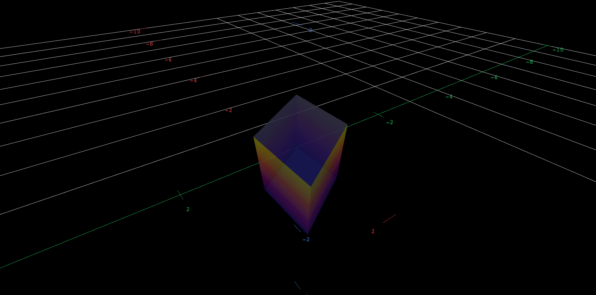
A translucent 3D parallelepiped spanned by the three column vectors (1,0,0), (a,1,0) and (0.4,0.3,1.2), drawn as six faces. Dragging the shear slider a from -1.5 to 1.5 makes the solid lean sideways like a stack of cards, but its volume stays exactly 1.2 - the absolute value of the determinant, unchanged by adding a multiple of one column to another. — The parallelepiped spanned by the columns u = (1, 0, 0), v = (a, 1, 0), w = (0.4, 0.3, 1.2). Drag the shear slider a: the solid leans, but its volume - the determinant, here 1.2 - never changes, because adding a multiple of one column to another leaves the determinant alone. The 3D sibling of the unit-square figure above.

There are a number of ways to define the determinant for an $n \times n$ matrix. Let us use the so-called cofactor expansion. We define $A_{i j}$ as the matrix $A$ with the $i^{th}$ row and the $j^{th}$ column deleted. For example, if

$If A = [\begin{matrix} 1 & 2 & 3 \\ 4 & 5 & 6 \\ 7 & 8 & 9 \end{matrix}], then A_{12} = [\begin{matrix} 4 & 6 \\ 7 & 9 \end{matrix}] and A_{23} = [\begin{matrix} 1 & 2 \\ 7 & 8 \end{matrix}] .$

We now define the determinant recursively

$det (A) \overset{def}{=} \sum_{j = 1}^{n} {(- 1)}^{1 + j} a_{1 j} det (A_{1 j}),$

or in other words

$\begin{matrix} + a_{1 n} det (A_{1 n}) if n is odd, \\ - a_{1 n} det (A_{1 n}) if n even. \end{matrix}$

For a

3 times 3

matrix, we get

det (A) = a_{11} det (A_{11}) - a_{12} det (A_{12}) + a_{13} det (A_{13})

. For example,

$\begin{matrix} det ([\begin{matrix} 1 & 2 & 3 \\ 4 & 5 & 6 \\ 7 & 8 & 9 \end{matrix}]) = 1 \cdot det ([\begin{matrix} 5 & 6 \\ 8 & 9 \end{matrix}]) - 2 \cdot det ([\begin{matrix} 4 & 6 \\ 7 & 9 \end{matrix}]) + 3 \cdot det ([\begin{matrix} 4 & 5 \\ 7 & 8 \end{matrix}]) \\ = 1 (5 \cdot 9 - 6 \cdot 8) - 2 (4 \cdot 9 - 6 \cdot 7) + 3 (4 \cdot 8 - 5 \cdot 7) = 0 . \end{matrix}$

It turns out that we did not have to necessarily use the first row. That is for any

i

$det (A) = \sum_{j = 1}^{n} {(- 1)}^{i + j} a_{i j} det (A_{i j}) .$

It is sometimes useful to use a row other than the first. In the following example it is more convenient to expand along the second row. Notice that for the second row we are starting with a negative sign.

$\begin{matrix} det ([\begin{matrix} 1 & 2 & 3 \\ 0 & 5 & 0 \\ 7 & 8 & 9 \end{matrix}]) = - 0 \cdot det ([\begin{matrix} 2 & 3 \\ 8 & 9 \end{matrix}]) + 5 \cdot det ([\begin{matrix} 1 & 3 \\ 7 & 9 \end{matrix}]) - 0 \cdot det ([\begin{matrix} 1 & 2 \\ 7 & 8 \end{matrix}]) \\ = 0 + 5 (1 \cdot 9 - 3 \cdot 7) + 0 = - 60 . \end{matrix}$

Let us check if it is really the same as expanding along the first row,

$\begin{matrix} det ([\begin{matrix} 1 & 2 & 3 \\ 0 & 5 & 0 \\ 7 & 8 & 9 \end{matrix}]) = 1 \cdot det ([\begin{matrix} 5 & 0 \\ 8 & 9 \end{matrix}]) - 2 \cdot det ([\begin{matrix} 0 & 0 \\ 7 & 9 \end{matrix}]) + 3 \cdot det ([\begin{matrix} 0 & 5 \\ 7 & 8 \end{matrix}]) \\ = 1 (5 \cdot 9 - 0 \cdot 8) - 2 (0 \cdot 9 - 0 \cdot 7) + 3 (0 \cdot 8 - 5 \cdot 7) = - 60 . \end{matrix}$

In computing the determinant, we alternately add and subtract the determinants of the submatrices

A_{i j}

multiplied by

a_{i j}

for a fixed

i

and all

j

. The numbers

{(- 1)}^{i + j} det (A_{i j})

are called cofactors of the matrix. And that is why this method of computing the determinant is called the cofactor expansion.

Similarly we do not need to expand along a row, we can expand along a column. For any $j$ ,

$det (A) = \sum_{i = 1}^{n} {(- 1)}^{i + j} a_{i j} det (A_{i j}) .$

A related fact is that

$det (A) = det (A^{T}) .$

A matrix is upper triangular if all elements below the main diagonal are

0

. For example,

$[ 1, 2, 3; 0, 5, 6; 0, 0, 9 ]$

is upper triangular. Similarly a lower triangular matrix is one where everything above the diagonal is zero. For example,

$[ 1, 0, 0; 4, 5, 0; 7, 8, 9 ].$

The determinant for triangular matrices is very simple to compute. Consider the lower triangular matrix. If we expand along the first row, we find that the determinant is 1 times the determinant of the lower triangular matrix

[ 5, 0; 8, 9 ]

. So the deteriminant is just the product of the diagonal entries:

$det ([\begin{matrix} 1 & 0 & 0 \\ 4 & 5 & 0 \\ 7 & 8 & 9 \end{matrix}]) = 1 \cdot 5 \cdot 9 = 45 .$

Similarly for upper triangular matrices

$det ([\begin{matrix} 1 & 2 & 3 \\ 0 & 5 & 6 \\ 0 & 0 & 9 \end{matrix}]) = 1 \cdot 5 \cdot 9 = 45 .$

In general, if

A

is triangular, then

$det open parenthesis A close parenthesis equals a sub 11 a sub 22 ⋯ a sub n n.$

A

is diagonal, then it is also triangular (upper and lower), so same formula applies. For example,

$det ([\begin{matrix} 2 & 0 & 0 \\ 0 & 3 & 0 \\ 0 & 0 & 5 \end{matrix}]) = 2 \cdot 3 \cdot 5 = 30 .$

In particular, the identity matrix

I

is diagonal, and the diagonal entries are all 1. Thus,

$det open parenthesis I close parenthesis equals 1.$

The determinant is telling you how geometric objects scale. If

B

doubles the sizes of geometric objects and

A

triples them, then

A B

(which applies

B

to an object and then it applies

A

) should make size go up by a factor of

6

. This is true in general:

This property is one of the most useful, and it is employed often to actually compute determinants. A particularly interesting consequence is to note what it means for the existence of inverses. Take $A$ and $B$ to be inverses, that is $A B = I$ . Then

$det (A) det (B) = det (A B) = det (I) = 1 .$

Neither

det (A)

nor

det (B)

can be zero. This fact is an extremely useful property of the determinant, and one which is used often in this book:

In fact, $det (A^{- 1}) det (A) = 1$ says that

$det (A^{- 1}) = \frac{1}{det (A)} .$

So we know what the determinant of

A^{- 1}

is without computing

A^{- 1}

Let us return to the formula for the inverse of a $2 times 2$ matrix:

$[^{\begin{matrix} a & b \\ c & d \end{matrix}] - 1} = \frac{1}{a d - b c} [\begin{matrix} d & - b \\ - c & a \end{matrix}] .$

Notice the determinant of the matrix

[ a, b; c, d ]

in the denominator of the fraction. The formula only works if the determinant is nonzero, otherwise we are dividing by zero.

A common notation for the determinant is a pair of vertical lines:

$| a, b; c, d | equals det open parenthesis [ a, b; c, d ] close parenthesis.$

Personally, I find this notation confusing as vertical lines usually mean a positive quantity, while determinants can be negative. Also think about how to write the absolute value of a determinant. This notation is not used in this book.

Adapted from Differential Equations for Engineers by Jiří Lebl (Oklahoma State University), hosted on LibreTexts (math.libretexts.org) and licensed under CC BY-SA 4.0. Changes were made. License: CC-BY-SA-4.0.