To do basic geometry, we need length, and we need angles. We have already seen the euclidean length, so let us figure out how to compute angles. Mostly, we are worried about the right angle1.
Given two (column) vectors in , we define the (standard) inner product as the dot product:
Why do we seemingly give a new notation for the dot product? Because there are other possible inner products, which are not the dot product, although we will not worry about others here. An inner product can even be defined on spaces of functions as we do in Chapter 4: But we digress.
The inner product satisfies the following rules:
, and if and only if ,
,
,
and .
Anything that satisfies the properties above can be called an inner product, although in this section we are concerned with the standard inner product in .
The standard inner product gives the euclidean length:
How does it give angles?
You may recall from multivariable calculus, that in two or three dimensions, the standard inner product (the dot product) gives you the angle between the vectors:
That is, is the angle that and make when they are based at the same point.
In (any dimension), we are simply going to say that from the formula is what the angle is. This makes sense as any two vectors based at the origin lie in a 2-dimensional plane (subspace), and the formula works in 2 dimensions. In fact, one could even talk about angles between functions this way, and we do in Chapter 4, where we talk about orthogonal functions (functions at right angle to each other).
To compute the angle we compute
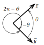
Our angles are always in radians. We are computing the cosine of the angle, which is really the best we can do. Given two vectors at an angle , we can give the angle as , , etc., see Figure . Fortunately, . If we solve for using the inverse cosine , we can just decree that .
Figure : Angle between vectors.
As we said, the most important angle is the right angle. A right angle is radians, and , so the formula is particularly easy in this case. We say vectors and are orthogonal if they are at right angles, that is if
The vectors and are orthogonal. So are and . However, and are not orthogonal as their inner product is and not .
Orthogonal Projection
A typical application of linear algebra is to take a difficult problem, write everything in the right basis, and in this new basis the problem becomes simple. A particularly useful basis is an orthogonal basis, that is a basis where all the basis vectors are orthogonal. When we draw a coordinate system in two or three dimensions, we almost always draw our axes as orthogonal to each other.
Generalizing this concept to functions, it is particularly useful in Chapter 4 to express a function using a particular orthogonal basis, the Fourier series.
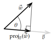
To express one vector in terms of an orthogonal basis, we need to first project one vector onto another. Given a nonzero vector , we define the orthogonal projection of onto as
For the geometric idea, see Figure . That is, we find the "shadow of " on the line spanned by if the direction of the sun’s rays were exactly perpendicular to the line. Another way of thinking about it is that the tip of the arrow of is the closest point on the line spanned by to the tip of the arrow of . In terms of euclidean distance, minimizes the distance among all vectors that are multiples of . Because of this, this projection comes up often in applied mathematics in all sorts of contexts we cannot solve a problem exactly: We can’t always solve "Find as a multiple of " but is the best "solution."
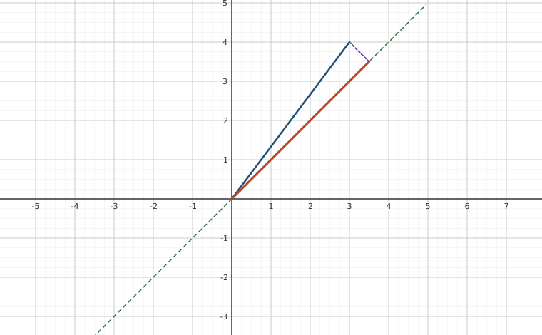
Interactive figureOrthogonal projection of w = (3, 4) onto vDrag the Direction of v slider from -1.5708 to 1.5708.
XYZ Graph · viewer build 5edf91b
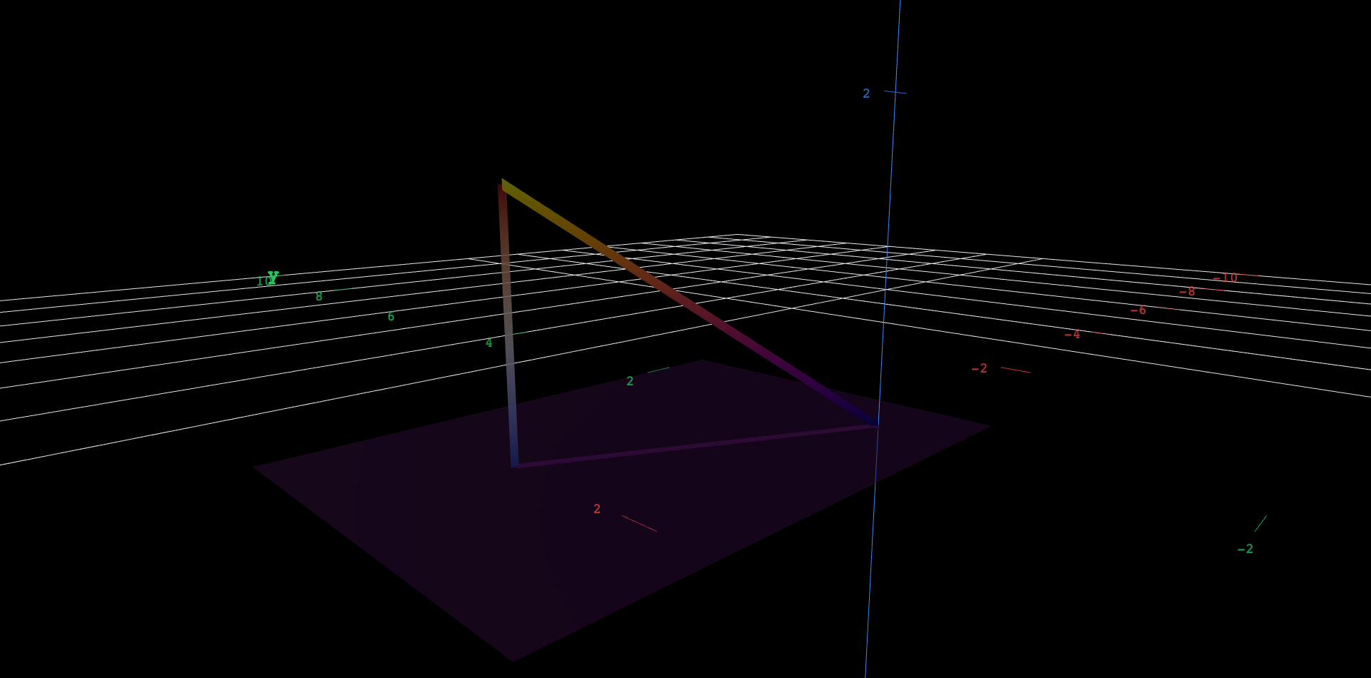
w = (3, 4) in blue, the line spanned by v dashed green, proj_v(w) in orange, and w − proj_v(w) dashed in purple — drawn from the tip of the projection to the tip of w, so the right angle is the one you can actually see. Drag the direction a to sweep the shadow along the line: the purple segment meets the green line at a right angle at every single setting, which is the check this section runs once by hand. At a = 0.7854 (π/4) the projection is (3.5, 3.5) = (7/2)·(1, 1) and at a = −0.7854 it is (−0.5, 0.5) = (−1/2)·(1, −1) — the very coefficients this section computes for (3, 4) in the orthogonal basis (1, 1), (1, −1). Push a past −0.64, where tan a = −3/4, and the projection collapses to a point, because there v ⟂ w and the shadow is nothing at all.Explore in 3D (opens in a new tab)The vector v = (2, 1, c) in orange, its orthogonal projection (2, 1, 0) onto the xy-plane in blue, and the perpendicular drop between them. Drag the slider for c: the projection never moves - projecting onto the plane simply discards the component orthogonal to it. At c = 0 there is nothing left to discard: v already lies in the plane, the drop shrinks to a point, and v is its own projection - the one setting where projecting changes nothing at all.Figure : Orthogonal projection.
The formula follows from basic trigonometry. The length of should be times the length of , that is . We take the unit vector in the direction of , that is, and we multiply it by the length of the projection. In other words,
Orthogonal Basis
As we said, a basis is an orthogonal basis if all vectors in the basis are orthogonal to each other, that is, if
for all choices of and where (a nonzero vector cannot be orthogonal to itself). A basis is furthermore called an orthonormal basis if all the vectors in a basis are also unit vectors, that is, if all the vectors have magnitude 1. For example, the standard basis is an orthonormal basis of : Any pair is orthogonal, and each vector is of unit magnitude.
The reason why we are interested in orthogonal (or orthonormal) bases is that they make it really simple to represent a vector (or a projection onto a subspace) in the basis. The simple formula for the orthogonal projection onto a vector gives us the coefficients. In Chapter 4, we use the same idea by finding the correct orthogonal basis for the set of solutions of a differential equation. We are then able to find any particular solution by simply applying the orthogonal projection formula, which is just a couple of a inner products.
Let us come back to linear algebra. Suppose that we have a subspace and an orthogonal basis . We wish to express in terms of the basis. If is not in the span of the basis (when it is not in the given subspace), then of course it is not possible, but the following formula gives us at least the orthogonal projection onto the subspace, or in other words, the best approximation in the subspace.
First suppose that is in the span. Then it is the sum of the orthogonal projections:
In other words, if we want to write , then Another way to derive this formula is to work in reverse. Suppose that . Take an inner product with , and use the properties of the inner product: As the basis is orthogonal, then whenever . That means that only one of the terms, the one, on the right hand side is nonzero and we get Solving for we find as before.
If the basis is orthonormal rather than orthogonal, then all the denominators are one. It is easy to make a basis orthonormal—divide all the vectors by their size. If you want to decompose many vectors, it may be better to find an orthonormal basis. In the example above, the orthonormal basis we would thus create is
Then the computation would have been Maybe the example is not so awe inspiring, but given vectors in rather than , then surely one would much rather do 20 inner products (or 40 if we did not have an orthonormal basis) rather than solving a system of twenty equations in twenty unknowns using row reduction of a matrix.
As we said above, the formula still works even if is not in the subspace, although then it does not get us the vector but its projection. More concretely, suppose that is a subspace that is the span of and is any vector. Let be the vector in that is the closest to . Then
Of course, if is in , then , as the closest vector in to is itself. But true utility is obtained when is not in . In much of applied mathematics, we cannot find an exact solution to a problem, but we try to find the best solution out of a small subset (subspace). The partial sums of Fourier series from Chapter 4 are one example. Another example is least square approximation to fit a curve to data. Yet another example is given by the most commonly used numerical methods to solve partial differential equations, the finite element methods.
Gram–Schmidt Process
Before leaving orthogonal bases, let us note a procedure for manufacturing them out of any old basis. It may not be difficult to come up with an orthogonal basis for a 2-dimensional subspace, but for a 20-dimensional subspace, it seems a daunting task. Fortunately, the orthogonal projection can be used to "project away" the bits of the vectors that are making them not orthogonal. It is called the Gram-Schmidt process.
We start with a basis of vectors . We construct an orthogonal basis as follows.
What we do is at the step, we take and we subtract the projection of to the subspace spanned by .
Footnotes
[1] When Euclid defined angles in his Elements, the only angle he ever really defined was the right angle.
These eBooks are a prerelease and are not yet certified conformant with WCAG 2.1 AA or ADA Title II. Every page is built against an automated accessibility gate, and the published editions will meet ADA Title II requirements when they release in late September 2026. If something is unusable, please tell us.

 Explore in 3D (opens in a new tab)