8.2 Stability and Classiﬁcation of Isolated Critical Points

Isolated Critical Points and Almost Linear Systems

A critical point is isolated if it is the only critical point in some small "neighborhood" of the point. That is, if we zoom in far enough it is the only critical point we see. In the above example, the critical point was isolated. If on the other hand there would be a whole curve of critical points, then it would not be isolated.

A system is called almost linear (at a critical point $open parenthesis x sub 0, y sub 0 close parenthesis$ ) if the critical point is isolated and the Jacobian at the point is invertible, or equivalently if the linearized system has an isolated critical point. In such a case, the nonlinear terms will be very small and the system will behave like its linearization, at least if we are close to the critical point.

In particular the system we have just seen in Examples 8.1.1 and 8.1.2 has two isolated critical points $open parenthesis 0, 0 close parenthesis$ and $open parenthesis 0, 1 close parenthesis$ , and is almost linear at both critical points as both of the Jacobian matrices $[ 0, 1; minus 1, 0 ]$ and $[ 0, 1; 1, 0 ]$ are invertible.

On the other hand a system such as $x^{'} = x^{2}$ , $y^{'} = y^{2}$ has an isolated critical point at $open parenthesis 0, 0 close parenthesis$ , however the Jacobian matrix

$[ 2 x, 0; 0, 2 y ]$

is zero when $open parenthesis x, y close parenthesis equals open parenthesis 0, 0 close parenthesis$ . Therefore the system is not almost linear. Even a worse example is the system $x^{'} = x$ , $y^{'} = x^{2}$ ,which does not have an isolated critical point, as $x^{'}$ and $y^{'}$ are both zero whenever $x equals 0$ , that is, the entire $y$ axis.

Fortunately, most often critical points are isolated, and the system is almost linear at the critical points. So if we learn what happens here, we have figured out the majority of situations that arise in applications.

Stability and Classification of Isolated Critical Points

Once we have an isolated critical point, the system is almost linear at that critical point, and we computed the associated linearized system, we can classify what happens to the solutions. We more or less use the classification for linear two-variable systems from Section 3.5, with one minor caveat. Let us list the behaviors depending on the eigenvalues of the Jacobian matrix at the critical point in Table $1$ . This table is very similar to Table 3.5.1, with the exception of missing “center” points. We will discuss centers later, as they are more complicated.

Table $1$ : Behavior of an almost linear system near an isolated critical point.
Eigenvalues of the Jacobian matrix	Behavior	Stability
real and both positive	source / unstable node	unstable
real and both negative	sink / stable node	asymptotically stable
real and opposite signs	saddle	unstable
complex with positive real part	spiral source	unstable
complex with negative real part	spiral sink	asymptotically stable

In the new third column, we have marked points as asymptotically stable or unstable. Formally, a stable critical point $open parenthesis x sub 0, y sub 0 close parenthesis$ is one where given any small distance $ϵ$ to $open parenthesis x sub 0, y sub 0 close parenthesis$ ,and any initial condition within a perhaps smaller radius around $open parenthesis x sub 0, y sub 0 close parenthesis$ ,the trajectory of the system will never go further away from $open parenthesis x sub 0, y sub 0 close parenthesis$ than $ϵ$ . An unstable critical point is one that is not stable. Informally, a point is stable if we start close to a critical point and follow a trajectory we will either go towards, or at least not get away from, this critical point.

A stable critical point $open parenthesis x sub 0, y sub 0 close parenthesis$ is called asymptotically stable if given any initial condition sufficiently close to $open parenthesis x sub 0, y sub 0 close parenthesis$ and any solution $(x (t), y (t))$ given that condition, then

$lim sub t → infinity open parenthesis x open parenthesis t close parenthesis, y open parenthesis t close parenthesis close parenthesis equals open parenthesis x sub 0, y sub 0 close parenthesis.$

That is, the critical point is asymptotically stable if any trajectory for a sufficiently close initial condition goes towards the critical point $open parenthesis x sub 0, y sub 0 close parenthesis$ .

Example 1

Consider $x^{'} = - y - x^{2}$ , $y^{'} = - x + y^{2}$ . See Figure $1$ for the phase diagram. Let us find the critical points. These are the points where $- y - x^{2} = 0$ and $- x + y^{2} = 0$ . The first equation means $y = - x^{2}$ , and so $y^{2} = x^{4}$ . Plugging into the second equation we obtain $- x + x^{4} = 0$ . Factoring we obtain $x (1 - x^{3}) = 0$ . Since we are looking only for real solutions we get either $x equals 0$ or $x equals 1$ . Solving for the corresponding $y$ using $y = - x^{2}$ ,we get two critical points, one being $open parenthesis 0, 0 close parenthesis$ and the other being $open parenthesis 1, minus 1 close parenthesis$ . Clearly the critical points are isolated. Let us compute the Jacobian matrix:

$[\begin{matrix} - 2 x & - 1 \\ - 1 & 2 y \end{matrix}] .$

At the point $open parenthesis 0, 0 close parenthesis$ we get the matrix $[\begin{matrix} 0 & - 1 \\ - 1 & 0 \end{matrix}]$ and so the two eigenvalues are $1$ and $minus 1$ . As the matrix is invertible, the system is almost linear at $open parenthesis 0, 0 close parenthesis$ . As the eigenvalues are real and of opposite signs, we get a saddle point, which is an unstable equilibrium point.

Figure

1

: The phase portrait with few sample trajectories of

x^{'} = - y - x^{2}

y^{'} = - x + y^{2}

At the point $open parenthesis 1, minus 1 close parenthesis$ we get the matrix $[\begin{matrix} - 2 & - 1 \\ - 1 & - 2 \end{matrix}]$ and computing the eigenvalues we get $minus 1$ , $minus 3$ .The matrix is invertible, and so the system is almost linear at $open parenthesis 1, minus 1 close parenthesis$ . As we have real eigenvalues both negative, the critical point is a sink, and therefore an asymptotically stable equilibrium point. That is, if we start with any point $(x_{i}, y_{i})$ close to $open parenthesis 1, minus 1 close parenthesis$ as an initial condition and plot a trajectory, it will approach $open parenthesis 1, minus 1 close parenthesis$ . In other words,

${lim}_{t \to \infty} (x (t), y (t)) = (1, - 1) .$

As you can see from the diagram, this behavior is true even for some initial points quite far from $open parenthesis 1, minus 1 close parenthesis$ ,but it is definitely not true for all initial points.

Example 2

Let us look at $x^{'} = y + y^{2} e^{x}$ , $y^{'} = x$ . First let us find the critical points. These are the points where $y + y^{2} e^{x} = 0$ and $x equals 0$ . Simplifying we get $0 = y + y^{2} = y (y + 1)$ . So the critical points are $open parenthesis 0, 0 close parenthesis$ and $open parenthesis 0, minus 1 close parenthesis$ ,and hence are isolated. Let us compute the Jacobian matrix:

$[\begin{matrix} y^{2} e^{x} & 1 + 2 y e^{x} \\ 1 & 0 \end{matrix}] .$

At the point $open parenthesis 0, 0 close parenthesis$ we get the matrix $[ 0, 1; 1, 0 ]$ and so the two eigenvalues are $1$ and $minus 1$ . As the matrix is invertible, the system is almost linear at $open parenthesis 0, 0 close parenthesis$ . And, as the eigenvalues are real and of opposite signs, we get a saddle point, which is an unstable equilibrium point.

At the point $open parenthesis 0, minus 1 close parenthesis$ we get the matrix $[ 1, minus 1; 1, 0 ]$ whose eigenvalues are $\frac{1}{2} \pm i \frac{\sqrt{3}}{2}$ . The matrix is invertible, and so the system is almost linear at $open parenthesis 0, minus 1 close parenthesis$ . As we have complex eigenvalues with positive real part, the critical point is a spiral source, and therefore an unstable equilibrium point.

Figure

2

: The phase portrait with few sample trajectories of

x^{'} = y + y^{2} e^{x}

y^{'} = x

See Figure $2$ for the phase diagram. Notice the two critical points, and the behavior of the arrows in the vector field around these points.

Trouble with Centers

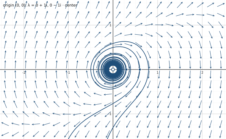
Recall, a linear system with a center meant that trajectories traveled in closed elliptical orbits in some direction around the critical point. Such a critical point we would call a center or a stable center. It would not be an asymptotically stable critical point, as the trajectories would never approach the critical point, but at least if you start sufficiently close to the critical point, you will stay close to the critical point. The simplest example of such behavior is the linear system with a center. Another example is the critical point $open parenthesis 0, 0 close parenthesis$ in Example 8.1.1.

The trouble with a center in a nonlinear system is that whether the trajectory goes towards or away from the critical point is governed by the sign of the real part of the eigenvalues of the Jacobian. Since this real part is zero at the critical point itself, it can have either sign nearby, meaning the trajectory could be pulled towards or away from the critical point.

Example 3

An easy example where such a problematic behavior is exhibited is the system $x^{'} = y, y^{'} = - x + y^{3}$ . The only critical point is the origin $open parenthesis 0, 0 close parenthesis$ . The Jacobian matrix is

$[ 0, 1; minus 1, 3 y squared ].$

At $open parenthesis 0, 0 close parenthesis$ the Jacobian matrix is $[ 0, 1; minus 1, 0 ]$ ,which has eigenvalues $\pm i$ . Therefore, the linearization has a center.

Using the quadratic equation, the eigenvalues of the Jacobian matrix at any point $(x, y)$ are

$λ = \frac{3}{2} y^{2} \pm i \frac{\sqrt{4 - 9 y^{4}}}{2} .$

At any point where $y ⧸ equals 0$ (so at most points near the origin), the eigenvalues have a positive real part ( $y^{2}$ can never be negative). This positive real part will pull the trajectory away from the origin. A sample trajectory for an initial condition near the origin is given in Figure $3$ .

$An unstable critical point (spiral source) at the origin for x'=y, y'=-x+y^{3}, even if the linearization has a center.$

Figure

3

: An unstable critical point (spiral source) at the origin for

x^{'} = y

y^{'} = - x + y^{3}

, even if the linearization has a center.

The moral of the example is that further analysis is needed when the linearization has a center. The analysis will in general be more complicated than in the above example, and is more likely to involve case-by-case consideration. Such a complication should not be surprising to you. By now in your mathematical career, you have seen many places where a simple test is inconclusive, perhaps starting with the second derivative test for maxima or minima, and requires more careful, and perhaps ad hoc analysis of the situation.

Function graph showing the direction field of the system x′ = y, y′ = -x+k*y^3, drawn from 308 sample arrows, and 2 trajectories through (0.3, 0) and (0.6, 0). Linearizing: origin (0, 0): λ = 0 + 1i, 0 − 1i · center. Adjustable parameter: Strength of the nonlinear term (k) = 1. Viewing window: x from -2.53 to 2.53, y from -1.57 to 1.57. — The section's own example x′ = y, y′ = −x + y³, with the cubic term on a slider so the true system and its linearization share one frame. The poster shows the book's case, k = 1. Pull k to 0 and the system becomes exactly the linearization at the origin, [[0, 1], [−1, 0]] with eigenvalues ±i, and both orbits close into perfect circles of radius 0.300 and 0.600. For any k > 0 they never close again: the orbit through (0.3, 0) comes back to 0.317 after one lap at k = 0.25, to 0.338 at k = 0.5, and to 0.396 at k = 1, gaining a little every lap until it spirals away. The Jacobian is [[0, 1], [−1, 3k·y²]], so Re λ = (3k/2)y² — the book's λ = (3/2)y² ± i·√(4 − 9y⁴)/2 at k = 1. That real part vanishes along the whole line y = 0 and is positive off it, and it grows with amplitude, which is why the wider orbit through (0.6, 0) breaks up at a far smaller k than the inner one. The readout linearizes at the origin: the cubic term contributes nothing there, so the linearization is a center — and a center is exactly the case the linearization cannot settle. Drag k and watch the trajectories spiral in or out while the readout keeps saying center.

Conservative Equations

An equation of the form

$x^{″} + f (x) = 0$

for an arbitrary function $f (x)$ is called a conservative equation. For example the pendulum equation is a conservative equation. The equations are conservative as there is no friction in the system so the energy in the system is "conserved." Let us write this equation as a system of nonlinear ODE.

$x^{'} = y, y^{'} = - f (x) .$

These types of equations have the advantage that we can solve for their trajectories easily. The trick is to first think of $y$ as a function of $x$ for a moment. Then use the chain rule

$x^{″} = y^{'} = y \frac{d y}{d x},$

where the prime indicates a derivative with respect to $t$ . We obtain $y \frac{d y}{d x} + f (x) = 0$ . We integrate with respect to $x$ to get $\int y \frac{d y}{d x} d x + \int f (x) d x = C$ . In other words

$\frac{1}{2} y^{2} + \int f (x) d x = C .$

We obtained an implicit equation for the trajectories, with different $C$ giving different trajectories. The value of $C$ is conserved on any trajectory. This expression is sometimes called the Hamiltonian or the energy of the system. If you look back to Section 1.8, you will notice that $y \frac{d y}{d x} + f (x) = 0$ is an exact equation, and we just found a potential function.

Example 4

Let us find the trajectories for the equation $x^{″} + x - x^{2} = 0$ , which is the equation from Example 8.1.1. The corresponding first order system is

$x^{'} = y, y^{'} = - x + x^{2} .$

Trajectories satisfy

$\frac{1}{2} y^{2} + \frac{1}{2} x^{2} - \frac{1}{3} x^{3} = C .$

We solve for $y$

$y = \pm \sqrt{- x^{2} + \frac{2}{3} x^{3} + 2 C} .$

Plotting these graphs we get exactly the trajectories in Figure 8.1.2. In particular we notice that near the origin the trajectories are closed curves: they keep going around the origin, never spiraling in or out. Therefore we discovered a way to verify that the critical point at $open parenthesis 0, 0 close parenthesis$ is a stable center. The critical point at $open parenthesis 0, 1 close parenthesis$ is a saddle as we already noticed. This example is typical for conservative equations.

Consider an arbitrary conservative equation. The trajectories are given by

$y = \pm \sqrt{- 2 \int f (x) d x + 2 C} .$

So all trajectories are mirrored across the $x$ -axis. In particular, there can be no spiral sources nor sinks. All critical points occur when $y equals 0$ (the $x$ -axis), that is when $x prime equals 0$ . The critical points are simply those points on the $x$ -axis where $f open parenthesis x close parenthesis equals 0$ . The Jacobian matrix is

$[ 0, 1; minus f prime open parenthesis x close parenthesis, 0 ].$

So the critical point is almost linear if $f prime open parenthesis x close parenthesis ⧸ equals 0$ at the critical point. Let $J$ denote the Jacobian matrix, then the eigenvalues of $J$ are solutions to

$0 = det (J - λ I) = λ^{2} + f^{'} (x) .$

Therefore $λ = \pm \sqrt{- f^{'} (x)}$ . In other words, either we get real eigenvalues of opposite signs, or we get purely imaginary eigenvalues. There are only two possibilities for critical points, either an unstable saddle point, or a stable center. There are never any asymptotically stable points, sinks, or sources.

Adapted from Differential Equations for Engineers by Jiří Lebl (Oklahoma State University), hosted on LibreTexts (math.libretexts.org) and licensed under CC BY-SA 4.0. Changes were made. License: CC-BY-SA-4.0.