8.5 Chaos

You have surely heard the story about the flap of a butterfly wing in the Amazon causing hurricanes in the North Atlantic. In a prior section, we mentioned that a small change in initial conditions of the planets can lead to very different configuration of the planets in the long term. These are examples of chaotic systems. Mathematical chaos is not really chaos, there is precise order behind the scenes. Everything is still deterministic. However a chaotic system is extremely sensitive to initial conditions. This also means even small errors induced via numerical approximation create large errors very quickly, so it is almost impossible to numerically approximate for long times. This is large part of the trouble as chaotic systems cannot be in general solved analytically.

Take the weather for example. As a small change in the initial conditions (the temperature at every point of the atmosphere for example) produces drastically different predictions in relatively short time, we cannot accurately predict weather. This is because we do not actually know the exact initial conditions, we measure temperatures at a few points with some error and then we somehow estimate what is in between. There is no way we can accurately measure the effects of every butterfly wing. Then we will solve numerically introducing new errors. That is why you should not trust weather prediction more than a few days out.

The idea of chaotic behavior was first noticed by Edward Lorenz in the 1960s when trying to model thermally induced air convection (movement). The equations Lorentz was looking at form the relatively simple looking system:

$x' = -10x +10y, \quad y' = 28x-y-xz, \quad z'=-\frac{8}{3}z + xy. \nonumber$

A small change in the initial conditions yield a very different solution after a reasonably short time.

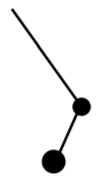
Picture of right down line segment to a point then connected by a down left line sigment to a larger point — Figure $\PageIndex{1}$

A very simple example the reader can experiment with, which displays chaotic behavior, is a double pendulum. The equations that govern this system are somewhat complicated and their derivation is quite tedious, so we will not bother to write them down. The idea is to put a pendulum on the end of another pendulum. If you look at the movement of the bottom mass, the movement will appear chaotic. This type of system is a basis for a whole number of office novelty desk toys. It is very simple to build a version. Take a piece of a string, and tie two heavy nuts at different points of the string; one at the end, and one a bit above. Now give the bottom nut a little push, as long as the swings are not too big and the string stays tight, you have a double pendulum system.

Duffing Equation and Strange Attractors

Let us study the so-called Duffing equation:

$x'' + a x' + bx + cx^3 = C \cos(\omega t). \nonumber$

Here $a$ , $b$ , $c$ , $C$ , and $\omega$ are constants. You will recognize that except for the $c x^3$ term, this equation looks like a forced mass-spring system. The $c x^3$ term comes up when the spring does not exactly obey Hooke's law (which no real-world spring actually does obey exactly). When $c$ is not zero, the equation does not have a nice closed form solution, so we have to resort to numerical solutions as is usual for nonlinear systems. Not all choices of constants and initial conditions will exhibit chaotic behavior. Let us study

$x''+0.05 x' + x^3 = 8\cos(t). \nonumber$

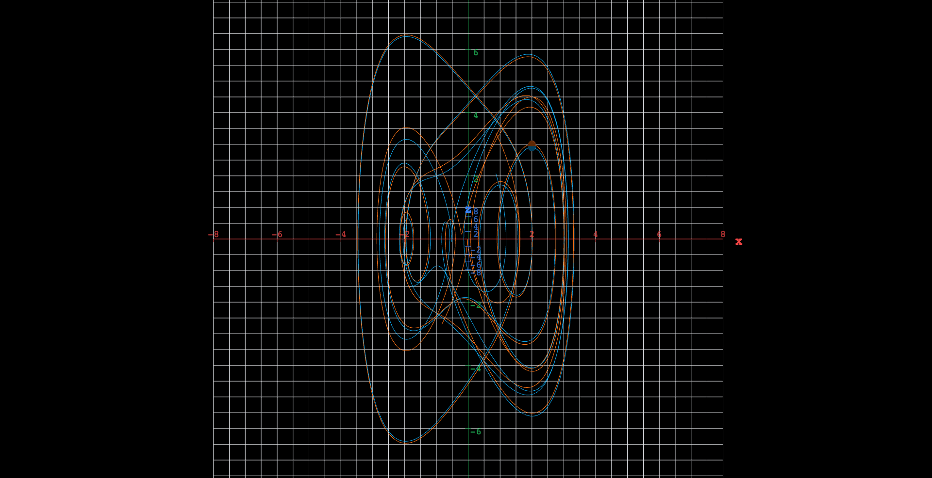
The equation is not autonomous, so we will not be able to draw the vector field in the phase plane. We can still draw the trajectories however. In Figure $\PageIndex{2}$ we plot trajectories for $t$ going from $0$ to $15$ , for two very close initial conditions $(2,3)$ and $(2,2.9)$ , and also the solutions in the $(x,t)$ space. The two trajectories are close at first, but after a while diverge significantly. This sensitivity to initial conditions is precisely what we mean by the system behaving chaotically.

Two looping curves in the phase plane, horizontal axis the position x from about -3.5 to 3.3 and vertical axis the velocity x-prime from about -6.5 to 6.5, drawn in orange and blue. Neither curve closes: each wanders through a band of overlapping loops filling most of the frame, the signature of a forced nonlinear oscillator that never repeats. The two curves begin at almost the same place, marked by a pair of dots near x = 2 with velocities 3 and 2.9, a tenth of a unit apart. They stay together at first -- still about a twentieth of a unit apart at t = 3 -- then drift measurably apart by t = 6 and end roughly one and a half units apart at t = 15, on different loops. The separation does not grow smoothly: it widens, narrows and widens again as the two solutions pass near each other. Either dot can be dragged to start the integration somewhere else. — Lebl's Duffing equation x'' + 0.05x' + x^3 = 8cos(t), drawn in the phase plane for his two initial conditions (2, 3) and (2, 2.9) -- a tenth of a unit apart in velocity. The equation is not autonomous, so there is no vector field to draw behind these curves, but the trajectories themselves tell the story: they track each other closely for the first few time units, then separate, and by t = 15 they are on different loops. Note that the gap does not widen steadily -- it narrows again around t = 9 before widening for good, which is why a single snapshot of the separation proves nothing. Each dot sits in the MIDDLE of its curve, not at one end: the renderer integrates both time directions from an initial condition, so tSpan [0, 15] draws t from −15 to +15. Everything described above is the forward half, running outward from the dots. The other half is the same two solutions followed backward, and they separate going that way too — sensitivity does not care which direction you run the clock. Drag either starting dot to test how little it takes to change the outcome.

Trajectories in phase space 0<=t<=15, for Duffing equation with initial conditions (2,3) and (2, 2.9). Solutions in (x,t)-space. — Figure $\PageIndex{2}$ : On left, two trajectories in phase space for $0\leq t\leq 15$ , for the Duffing equation one with initial conditions $(2,3)$ and the other with $(2, 2.9)$ . On right the two solutions in $(x,t)$ -space.

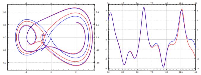
Let us see the long term behavior. In Figure $\PageIndex{3}$ , we plot the behavior of the system for initial conditions $(2,3)$ , but for much longer period of time. Note that for this period of time it was necessary to use a ridiculously large number of steps1 in the numerical algorithm used to produce the graph, as even small errors quickly propagate. From the graph it is hard to see any particular pattern in the shape of the solution except that it seems to oscillate, but each oscillation appears quite unique. The oscillation is expected due to the forcing term.

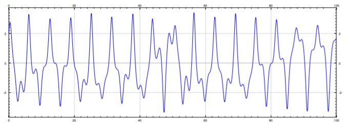
The solution to the given Duffing equation for t from 0 to 100. — Figure $\PageIndex{3}$ : The solution to the given Duffing equation for $t$ from $0$ to $100$ .

In general it is very difficult to analyze chaotic systems, or to find the order behind the madness, but let us try to do something that we did for the standard mass-spring system. One way we analyzed what happens is that we figured out what was the long term behavior (not dependent on initial conditions). From the figure above it is clear that we will not get a nice description of the long term behavior, but perhaps we can figure out some order to what happens on each "oscillation" and what do these oscillations have in common.

The concept we will explore is that of a Poincaré section2. Instead of looking at $t$ in a certain interval, we will look at where the system is at a certain sequence of points in time. Imagine flashing a strobe at a certain fixed frequency and drawing the points where the solution is during the flashes. The right strobing frequency depends on the system in question. The correct frequency to use for the forced Duffing equation (and other similar systems) is the frequency of the forcing term. For the Duffing equation above, find a solution $\bigl(x(t),y(t)\bigr)$ , and look at the points

$\bigl(x(0),y(0)\bigr), \quad \bigl(x(2\pi),y(2\pi)\bigr), \quad \bigl(x(4\pi),y(4\pi)\bigr), \quad \bigl(x(6\pi),y(6\pi)\bigr), \quad \ldots \nonumber$

As we are really not interested in the transient part of the solution, that is, the part of the solution that depends on the initial condition we skip some number of steps in the beginning. For example, we might skip the first 100 such steps and start plotting points at $t = 100(2\pi)$ , that is

$\bigl(x(200\pi),y(200\pi)\bigr), \quad \bigl(x(202\pi),y(202\pi)\bigr), \quad \bigl(x(204\pi),y(204\pi)\bigr), \quad \bigl(x(206\pi),y(206\pi)\bigr), \quad \ldots \nonumber$

The plot of these points is the Poincaré section. After plotting enough points, a curious pattern emerges in Figure $\PageIndex{4}$ (the left hand picture), a so-called strange attractor.

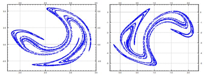
Strange attractor. The left plot is with no phase shift, the right plot has phase shift pi/4. — Figure $\PageIndex{4}$ : Strange attractor. The left plot is with no phase shift, the right plot has phase shift $\frac{\pi}{4}$ .

If we have a sequence of points, then an attractor is a set towards which the points in the sequence eventually get closer and closer to, that is, they are attracted. The Poincaré section above is not really the attractor itself, but as the points are very close to it, we can see its shape. The strange attractor in the figure is a very complicated set, and it in fact has fractal structure, that is, if you would zoom in as far as you want, you would keep seeing the same complicated structure.

The initial condition does not really make any difference. If we started with different initial condition, the points would eventually gravitate towards the attractor, and so as long as we throw away the first few points, we always get the same picture.

An amazing thing is that a chaotic system such as the Duffing equation is not random at all. There is a very complicated order to it, and the strange attractor says something about this order. We cannot quite say what state the system will be in eventually, but given a fixed strobing frequency we can narrow it down to the points on the attractor.

If you would use a phase shift, for example $\frac{\pi}{4}$ , and look at the times

$\frac{\pi}{4}, \quad 2\pi+\frac{\pi}{4}, \quad 4\pi+\frac{\pi}{4}, \quad 6\pi+\frac{\pi}{4}, \quad \ldots \nonumber$

you would obtain a slightly different looking attractor. The picture is the right hand side of Figure $\PageIndex{4}$ . It is as if we had rotated, distorted slightly, and then moved the original. Therefore for each phase shift you can find the set of points towards which the system periodically keeps coming back to.

You should study the pictures and notice especially the scales---where are these attractors located in the phase plane. Notice the regions where the strange attractor lives and compare it to the plot of the trajectories in Figure $\PageIndex{2}$ .

Let us compare the discussion in this section to the discussion in Section 2.6 about forced oscillations. Take the equation

$x''+2p x' + \omega_0^2 x = \frac{F_0}{m} \cos (\omega t). \nonumber$

This is like the Duffing equation, but with no $x^3$ term. The steady periodic solution is of the form

$x = C \cos (\omega t + \gamma). \nonumber$

Strobing using the frequency $\omega$ we would obtain a single point in the phase space. So the attractor in this setting is a single point---an expected result as the system is not chaotic. In fact it was the opposite of chaotic. Any difference induced by the initial conditions dies away very quickly, and we settle into always the same steady periodic motion.

Lorenz System

In two dimensions to have the kind of chaotic behavior we are looking for, we have to study forced, or non-autonomous, systems such as the Duffing equation. Due to the Poincaré-Bendoxson Theorem, if an autonomous two-dimensional system has a solution that exists for all time in the future and does not go towards infinity, then we obtain a limit cycle or a closed trajectory. Hardly the chaotic behavior we are looking for.

In three dimensions even autonomous systems can be chaotic. Let us very briefly return to the Lorenz system

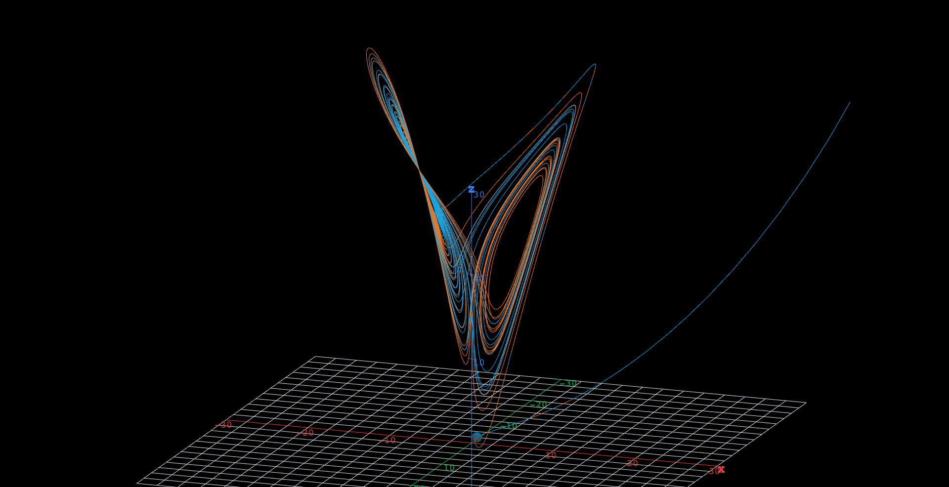
$x' = -10x +10y, \qquad y' = 28x-y-xz, \qquad z'=-\frac{8}{3}z + xy. \nonumber$

The Lorenz system is an autonomous system in three dimensions exhibiting chaotic behavior. See the Figure $\PageIndex{5}$ for a sample trajectory, which is now a curve in three-dimensional space.

A three-dimensional curve traced twice over, in orange and blue, forming the Lorenz attractor: two spiral lobes meeting in a V, the left lobe leaning up and away and the right lobe opening toward the viewer, together making the shape usually called the butterfly. Both curves wind many turns around one lobe, cross over near the middle, wind around the other, and switch about eleven times over the run without ever closing into a repeating loop. The shape rises from the horizontal xy grid at the bottom to about z = 48 at the top, and spans roughly x = -17 to 20 and y = -23 to 27. The two solutions start from a single dot on the grid near the origin, one thousandth of a unit apart, and are drawn on top of one another for the first half of the run -- still within a sixth of a unit at t = 15. Shortly before t = 20 they separate and finish on opposite lobes, after which they wander the same shape independently, sometimes near each other again and sometimes far apart, rather than drifting steadily further apart. A single thin blue strand leaves the butterfly toward the lower right and runs off the edge of the picture: that is the same solution followed BACKWARD in time, which does not stay on the attractor but escapes -- the attractor pulls solutions in only as time runs forward. Either starting dot can be dragged to re-integrate from a new initial condition. — The Lorenz system x' = -10x + 10y, y' = 28x - y - xz, z' = -8/3 z + xy, integrated from two starting points that differ by one thousandth in z alone. For the first fifteen time units the two solutions are a single visible curve; shortly before t = 20 they split and finish on opposite wings. After the split the distance between them does not keep growing -- both are trapped on the same bounded attractor, so they simply wander over it independently. That is what sensitivity to initial conditions looks like: not an explosion, but a total loss of any ability to say which wing the solution is on. The one thin strand running off to the lower right is the same solution followed backward in time; it escapes rather than settling, because the attractor attracts only forward in time. Drag either starting point, or orbit the figure, to see that the butterfly is the same from any start.

Graph of a trajectory in the Lorenz system. — Figure $\PageIndex{5}$ : A trajectory in the Lorenz system.

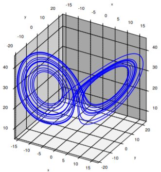
The solutions will tend to an attractor in space, the so-called Lorenz attractor. In this case no strobing is necessary. Again we cannot quite see the attractor itself, but if we try to follow a solution for long enough, as in the figure, we will get a pretty good picture of what the attractor looks like. The Lorenz attractor is also a strange attractor and has a complicated fractal structure. And, just as for the Duffing equation, what we want to draw is not the whole trajectory, but start drawing the trajectory after a while, once it is close to the attractor.

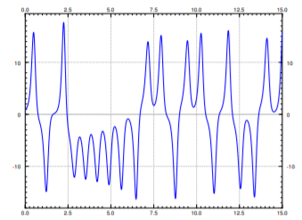
The path is not just a repeating figure-eight. The trajectory will spin some seemingly random number of times on the left, then spin a number of times on the right, and so on. As this system arose in weather prediction, one can perhaps imagine a few days of warm weather and then a few days of cold weather, where it is not easy to predict when the weather will change, just as it is not really easy to predict far in advance when the solution will jump onto the other side. See Figure $\PageIndex{6}$ for a plot of the $x$ component of the solution drawn above. A negative $x$ corresponds to the left "loop" and a positive $x$ corresponds to the right "loop".

Graph of the x(t) component of the solution. — Figure $\PageIndex{6}$ : Graph of the $x(t)$ component of the solution.

Most of the mathematics we studied in this book is quite classical and well understood. On the other hand, chaos, including the Lorenz system, continues to be the subject of current research. Furthermore, chaos has found applications not just in the sciences, but also in art.

Footnotes

[1] In fact for reference, 30,000 steps were used with the Runge–Kutta algorithm, see exercises in Section 1.7.

[2] Named for the French polymath Jules Henri Poincaré (1854-1912).

Adapted from Differential Equations for Engineers by Jiří Lebl (https://www.jirka.org/diffyqs/), © Jiří Lebl, licensed under CC BY-SA 4.0. Changes were made. License: CC-BY-SA-4.0.