2.4 Mechanical Vibrations

Let us look at some applications of linear second order constant coefficient equations.

Some examples

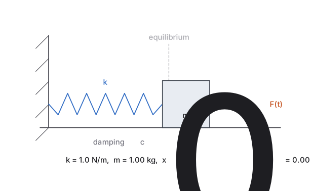
Diagram of a forced, damped mass-spring system: a hatched wall, spring k, block m, damping c on the surface, and an arrow F of t driving the block to the right. — Figure $1$

Our first example is a mass on a spring. Suppose we have a mass $m greater than 0$ (in kilograms) connected by a spring with spring constant $k greater than 0$ (in newtons per meter) to a fixed wall. There may be some external force $F (t)$ (in newtons) acting on the mass. Finally, there is some friction measured by $c greater than or equal to 0$ (in newton-seconds per meter) as the mass slides along the floor (or perhaps there is a damper connected).

Let $x$ be the displacement of the mass ( $x equals 0$ is the rest position), with $x$ growing to the right (away from the wall). The force exerted by the spring is proportional to the compression of the spring by Hooke’s law. Therefore, it is $k x$ in the negative direction. Similarly the amount of force exerted by friction is proportional to the velocity of the mass. By Newton’s second law we know that force equals mass times acceleration and hence $m x^{″} = F (t) - c x^{'} - k x$ or

$m x^{″} + c x^{'} + k x = F (t)$

This is a linear second order constant coefficient ODE. We set up some terminology about this equation. We say the motion is

forced, if $F ≢ 0$ (if $F$ is not identically zero),
unforced or free, if $F ≡ 0$ (if $F$ is identically zero),
damped, if $c greater than 0$ , and
undamped, if $c equals 0$ .

This system appears in lots of applications even if it does not at first seem like it. Many real-world scenarios can be simplified to a mass on a spring. For example, a bungee jump setup is essentially a mass and spring system (you are the mass). It would be good if someone did the math before you jump off the bridge, right? Let us give two other examples.

Here is an example for electrical engineers. Consider the pictured $R L C$ circuit. There is a resistor with a resistance of $R$ ohms, an inductor with an inductance of $L$ henries, and a capacitor with a capacitance of $C$ farads. There is also an electric source (such as a battery) giving a voltage of $E (t)$ volts at time $t$ (measured in seconds). Let $Q (t)$ be the charge in coulombs on the capacitor and $I (t)$ be the current in the circuit. The relation between the two is $Q^{'} = I$ . By elementary principles we find $L I^{'} + R I + \frac{Q}{C} = E$ . We differentiate to get

$L I^{″} (t) + R I^{'} (t) + \frac{1}{C} I (t) = E^{'} (t) .$

Diagram of a series circuit loop with a voltage source E, capacitor C, inductor L and resistor R in turn, so one current flows through all four. — Figure $2$

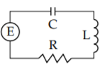
This is a nonhomogeneous second order constant coefficient linear equation. As $L, R$ , and $C$ are all positive, this system behaves just like the mass and spring system. Position of the mass is replaced by current. Mass is replaced by inductance, damping is replaced by resistance, and the spring constant is replaced by one over the capacitance. The change in voltage becomes the forcing function—for constant voltage this is an unforced motion.

Our next example behaves like a mass and spring system only approximately. Suppose a mass $m$ hangs on a pendulum of length $L$ . We seek an equation for the angle $θ (t)$ (in radians). Let $g$ be the force of gravity. Elementary physics mandates that the equation is

$θ^{″} + \frac{g}{L} \sin θ = 0 .$

Force diagram of a pendulum: rod of length L swung right of vertical by angle theta, bob m on an arc, with arrows for gravity m g, the tangential component m g sine theta, and m L theta double-prime opposing it. — Figure $3$

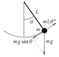
Let us derive this equation using Newton's second law: force equals mass times acceleration. The acceleration is $L θ^{″}$ and mass is $m$ . So $m L θ^{″}$ has to be equal to the tangential component of the force given by the gravity, which is $m g \sin θ$ in the opposite direction. So $m L θ^{″} = - m g \sin θ$ . The $m$ curiously cancels from the equation.

Now we make our approximation. For small $θ$ we have that approximately $\sin θ \approx θ$ . This can be seen by looking at the graph. In Figure $4$ we can see that for approximately $minus 0.5 less than θ less than 0.5$ (in radians) the graphs of $\sin θ$ and $θ$ are almost the same.

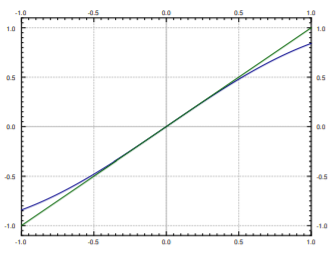
Plot of a green line of slope 1 and a blue curve on axes from -1 to 1; the two are indistinguishable between about -0.5 and 0.5, and the blue ends near 0.84 at angle 1. — Figure $4$ : The graphs of $\sin θ$ and $θ$ (in radians).

Therefore, when the swings are small, $θ$ is small and we can model the behavior by the simpler linear equation

$θ^{″} + \frac{g}{L} θ = 0 .$

The errors from this approximation build up. So after a long time, the state of the real-world system might be substantially different from our solution. Also we will see that in a mass-spring system, the amplitude is independent of the period. This is not true for a pendulum. Nevertheless, for reasonably short periods of time and small swings (that is, only small angles $θ$ ), the approximation is reasonably good.

In real-world problems it is often necessary to make these types of simplifications. We must understand both the mathematics and the physics of the situation to see if the simplification is valid in the context of the questions we are trying to answer.

Free Undamped Motion

In this section we will only consider free or unforced motion, as we cannot yet solve nonhomogeneous equations. Let us start with undamped motion where $c equals 0$ . We have the equation

$m x^{″} + k x = 0$

If we divide by $m$ and let $w_{0} = \sqrt{\frac{k}{m}}$ , then we can write the equation as

$x^{″} + w_{0}^{2} x = 0$

The general solution to this equation is

$x (t) = A \cos (w_{0} t) + B \sin (w_{0} t)$

By a trigonometric identity, we have that for two different constants $C$ and $γ$ , we have

$A \cos (w_{0} t) + B \sin (w_{0} t) = C \cos (w_{0} t - γ)$

It is not hard to compute that $C = \sqrt{A^{2} + B^{2}}$ and $\tan γ = \frac{B}{A}$ . Therefore, we let $C$ and $γ$ be our arbitrary constants and write $x (t) = C \cos (w_{0} t - γ)$ .

While it is generally easier to use the first form with $A$ and $B$ to solve for the initial conditions, the second form is much more natural. The constants $C$ and $γ$ have very nice interpretation. We look at the form of the solution

$x (t) = C \cos (w_{0} t - γ)$

We can see that the amplitude is $C$ , $w sub 0$ is the (angular) frequency, and $γ$ is the so-called phase shift. The phase shift just shifts the graph left or right. We call $w sub 0$ the natural (angular) frequency. This entire setup is usually called simple harmonic motion.

Let us pause to explain the word angular before the word frequency. The units of $w sub 0$ are radians per unit time, not cycles per unit time as is the usual measure of frequency. Because we know one cycle is $2 π$ radians, the usual frequency is given by $\frac{w_{0}}{2 π}$ . It is simply a matter of where we put the constant $2 π$ , and that is a matter of taste.

The period of the motion is one over the frequency (in cycles per unit time) and hence $\frac{2 π}{w_{0}}$ . That is the amount of time it takes to complete one full oscillation.

Example 1

Suppose that $m equals 2 k g$ and $k = 8 \frac{N}{m}$ . The whole mass and spring setup is sitting on a truck that was traveling at $1 \frac{m}{s}$ . The truck crashes and hence stops. The mass was held in place $0.5$ meters forward from the rest position. During the crash the mass gets loose. That is, the mass is now moving forward at $1 \frac{m}{s}$ , while the other end of the spring is held in place. The mass therefore starts oscillating. What is the frequency of the resulting oscillation and what is the amplitude. The units are the mks units (meters-kilograms-seconds).

The setup means that the mass was at half a meter in the positive direction during the crash and relative to the wall the spring is mounted to, the mass was moving forward (in the positive direction) at $1 \frac{m}{s}$ . This gives us the initial conditions.

So the equation with initial conditions is

$2 x^{″} + 8 x = 0, x (0) = 0.5, x^{'} (0) = 1$

We can directly compute $w_{0} = \sqrt{\frac{k}{m}} = \sqrt{4} = 2$ . Hence the angular frequency is 2. The usual frequency in Hertz (cycles per second) is $\frac{2}{2 π} = \frac{1}{π} \approx 0.318$ .

The general solution is

$x (t) = A \cos (2 t) + B \sin (2 t)$

Letting $x open parenthesis 0 close parenthesis equals 0.5$ means $A equals 0.5$ . Then $x^{'} (t) = - 2 (0.5) \sin (2 t) + 2 B \cos (2 t)$ . Letting $x prime open parenthesis 0 close parenthesis equals 1$ we get $B equals 0.5$ . Therefore, the amplitude is $C = \sqrt{A^{2} + B^{2}} = \sqrt{0.25 + 0.25} = \sqrt{0.5} \approx 0.707$ . The solution is

$x (t) = 0.5 \cos (2 t) + 0.5 \sin (2 t)$

A plot of $x (t)$ is shown in Figure $5$ .

Figure

5

: Simple undamped oscillation.

In general, for free undamped motion, a solution of the form

$x (t) = A \cos (w_{0} t) + B \sin (w_{0} t)$

corresponds to the initial conditions $x open parenthesis 0 close parenthesis equals A$ and $x prime open parenthesis 0 close parenthesis equals w sub 0 B$ . Therefore, it is easy to figure out $A$ and $B$ from the initial conditions. The amplitude and the phase shift can then be computed from $A$ and $B$ . In the example, we have already found the amplitude $C$ . Let us compute the phase shift. We know that $\tan γ = \frac{B}{A} = 1$ . We take the arctangent of 1 and get approximately 0.785. We still need to check if this $γ$ is in the correct quadrant (and add $π$ to $γ$ if it is not). Since both $A$ and $B$ are positive, then $γ$ should be in the first quadrant, and 0.785 radians really is in the first quadrant.

Free Damped Motion

Let us now focus on damped motion. Let us rewrite the equation

$m x^{″} + c x^{'} + k x = 0$

$x^{″} + 2 p x^{'} + w_{0}^{2} x = 0$

where

$w_{0} = \sqrt{\frac{k}{m}}, p = \frac{c}{2 m}$

The characteristic equation is

$r^{2} + 2 p r + w_{0}^{2} = 0$

Using the quadratic formula we get that the roots are

$r = - p \pm \sqrt{p^{2} - w_{0}^{2}}$

The form of the solution depends on whether we get complex or real roots. We get real roots if and only if the following number is nonnegative:

$p^{2} - w_{0}^{2} = {(\frac{c}{2 m})}^{2} - \frac{k}{m} = \frac{c^{2} - 4 k m}{4 m^{2}}$

The sign of $p squared minus w 0 2$ is the same as the sign of $c squared minus 4 k m$ . Thus we get real roots if and only if $c squared minus 4 k m$ is nonnegative, or in other words if $c squared greater than or equal to 4 k m$ .

Overdamping

When $c squared minus 4 k m greater than 0$ , we say the system is overdamped. In this case, there are two distinct real roots $r sub 1$ and $r sub 2$ . Notice that both roots are negative. As $\sqrt{p^{2} - w_{0}^{2}}$ is always less than $P$ , then $- P \pm \sqrt{P^{2} - w_{0}^{2}}$ is negative.

The solution is

$x (t) = C_{1} e^{r_{1} t} + C_{2} e^{r_{2} t}$

Since $r sub 1, r sub 2$ are negative, $x open parenthesis t close parenthesis → 0$ as $t \to \infty$ . Thus the mass will tend towards the rest position as time goes to infinity. For a few sample plots for different initial conditions (Figure $6$ ).

Three solution curves over time 0 to 100, all starting at 1 and settling to zero without oscillating: blue first rises to about 1.57, green falls monotonically, red dips to about -0.13. — Figure $6$ : Overdamped motion for several different initial conditions.

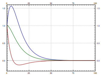
Do note that no oscillation happens. In fact, the graph will cross the $x$ axis at most once. To see why, we try to solve $0 = C_{1} e^{r_{1} t} + C_{2} e^{r_{2} t}$ . Therefore, $C_{1} e^{r_{1} t} = - C_{2} e^{r_{2} t}$ and using laws of exponents we obtain

$\frac{- C_{1}}{C_{2}} = e^{(r_{2} - r_{1}) t}$

This equation has at most one solution $t greater than or equal to 0$ . For some initial conditions the graph will never cross the $x$ axis, as is evident from the sample graphs.

Example 2

Suppose the mass is released from rest. That is $x open parenthesis 0 close parenthesis equals x sub 0$ and $x prime open parenthesis 0 close parenthesis equals 0$ . Then

$x (t) = \frac{x_{0}}{r_{1} - r_{2}} (r_{1} e^{r_{2} t} - r_{2} e^{r_{1} t})$

It is not hard to see that this satisfies the initial conditions.

Critical damping

When $c^{2} - 4 k m = 0$ , we say the system is critically damped. In this case, there is one root of multiplicity 2 and this root is $- P$ . Therefore, our solution is

$x (t) = C_{1} e^{- p t} + C_{2} t e^{- p t}$

The behavior of a critically damped system is very similar to an overdamped system. After all a critically damped system is in some sense a limit of overdamped systems. Since these equations are really only an approximation to the real world, in reality we are never critically damped, it is a place we can only reach in theory. We are always a little bit underdamped or a little bit overdamped. It is better not to dwell on critical damping.

Underdamping

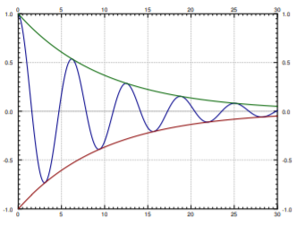
Plot of a blue underdamped oscillation over time 0 to 30 starting at 1, period about 6.3, peaks shrinking through 0.53, 0.29, 0.17 and 0.09 between green and red exponential envelopes. — Figure $7$ : Underdamped motion with the envelope curves shown.

When $c squared minus 4 k m less than 0$ , we say the system is underdamped. In this case, the roots are complex.

$\begin{matrix} r = - p \pm \sqrt{p^{2} - w_{0}^{2}} \\ = - p \pm \sqrt{- 1} \sqrt{w_{0}^{2} - p^{2}} \\ = - p \pm i w_{1} \end{matrix}$

where $w_{1} = \sqrt{w_{0}^{2} - p^{2}}$ . Our solution is

$x (t) = e^{- p t} (A \cos (w_{1} t) + B \sin (w_{1} t)$

$x (t) = C e^{- p t} \cos (w_{1} t - γ)$

An example plot is given in Figure $7$ . Note that we still have that $x open parenthesis t close parenthesis → 0$ as $t \to \infty$ .

In the figure we also show the envelope curves $C e^{- p t}$ and $- C e^{p t}$ . The solution is the oscillating line between the two envelope curves. The envelope curves give the maximum amplitude of the oscillation at any given point in time. For example if you are bungee jumping, you are really interested in computing the envelope curve so that you do not hit the concrete with your head.

Function graph showing y = 3*exp(-c*x/2)*cos(sqrt(1-c^2/4)*x) on x in [0, 12], y = 3*exp(-c*x/2)*cosh(sqrt(c^2/4-1)*x) on x in [0, 12], y = 3*exp(-c*x/2) + 0*sqrt(1-c^2/4) on x in [0, 12] and y = -3*exp(-c*x/2) + 0*sqrt(1-c^2/4) on x in [0, 12]. Adjustable parameter: Damping c (c) = 0.5 N·s/m. Viewing window: x from -0.33 to 12.13, y from -3.85 to 3.85. — Free motion for m = k = 1, so p = c/2 and w0 = 1. The solid curve is x(t) = 3e^(-pt)cos(w1 t) with w1 = sqrt(1 - c^2/4); the dashed curves are the envelopes +/-3e^(-pt), and because the phase shift is 0 the envelope touches the solution at every crest. Slide c down to 0 and the envelopes flatten into horizontal lines and the curve becomes the simple undamped oscillation of Figure 5. Raise c and w1 shrinks, exactly as the text predicts, until at c = 2 (c^2 = 4km) the upper envelope has collapsed onto the solution; past that the cosine becomes a cosh, the envelopes drop away, and what is left is the non-oscillating decay of Figure 6.

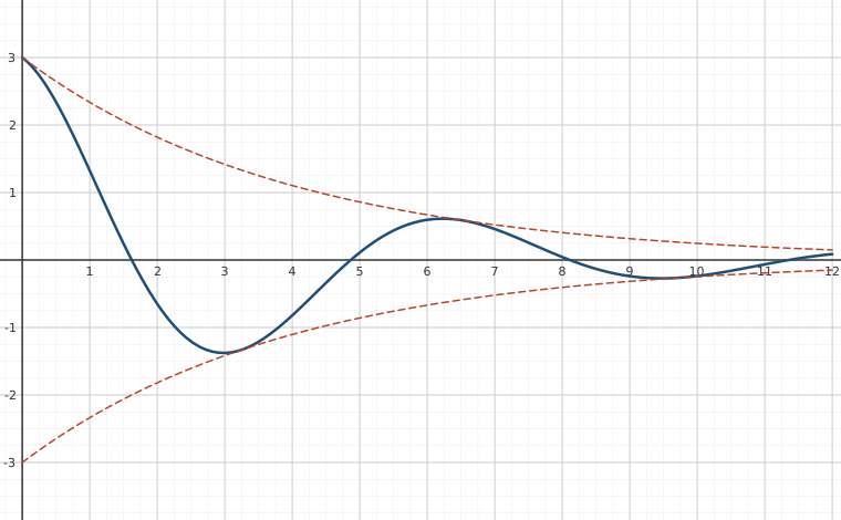
The phase shift $γ$ just shifts the graph left or right but within the envelope curves (the envelope curves do not change if $γ$ changes).

Finally note that the angular pseudo-frequencyto the power 1(we do not call it a frequency since the solution is not really a periodic function) $w sub 1$ becomes smaller when the damping $c$ (and hence $P$ ) becomes larger. This makes sense. When we change the damping just a little bit, we do not expect the behavior of the solution to change dramatically. If we keep making $c$ larger, then at some point the solution should start looking like the solution for critical damping or overdamping, where no oscillation happens. So if $c^{2}$ approaches $4 k m$ , we want $w sub 1$ to approach 0.

On the other hand when $c$ becomes smaller, $w sub 1$ approaches $w sub 0$ ( $w sub 1$ is always smaller than $w sub 0$ ), and the solution looks more and more like the steady periodic motion of the undamped case. The envelope curves become flatter and flatter as $c$ (and hence $P$ ) goes to 0.

Footnotes

[1] We do not call $ω sub 1$ a frequency since the solution is not really a periodic function.

Adapted from Differential Equations for Engineers by Jiří Lebl (Oklahoma State University), hosted on LibreTexts (math.libretexts.org) and licensed under CC BY-SA 4.0. Changes were made. License: CC-BY-SA-4.0.