
18.5 Electric Field Lines: Multiple Charges
Learning Objectives
By the end of this section, you will be able to:
- Calculate the total force (magnitude and direction) exerted on a test charge from more than one charge
- Describe an electric field diagram of a positive point charge; of a negative point charge with twice the magnitude of positive charge
- Draw the electric field lines between two points of the same charge; between two points of opposite charge.
Drawings using lines to represent electric fields around charged objects are very useful in visualizing field strength and direction. Since the electric field has both magnitude and direction, it is a vector. Like all vectors, the electric field can be represented by an arrow that has length proportional to its magnitude and that points in the correct direction. (We have used arrows extensively to represent force vectors, for example.)
Figure 18.22 shows two pictorial representations of the same electric field created by a positive point charge . Figure 18.22 (b) shows the standard representation using continuous lines. Figure 18.22 (a) shows numerous individual arrows with each arrow representing the force on a test charge . Field lines are essentially a map of infinitesimal force vectors.
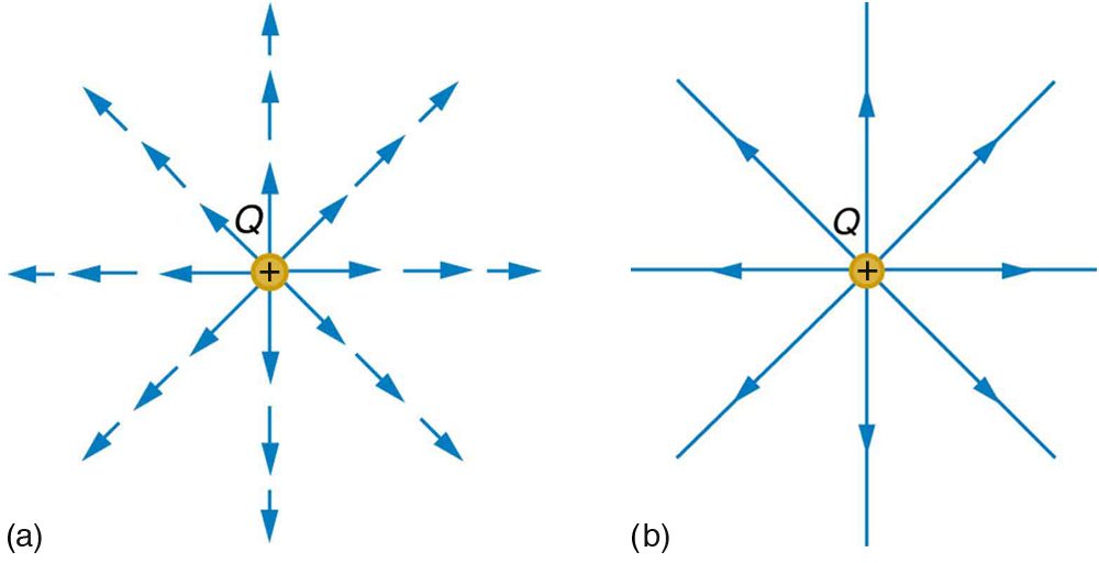
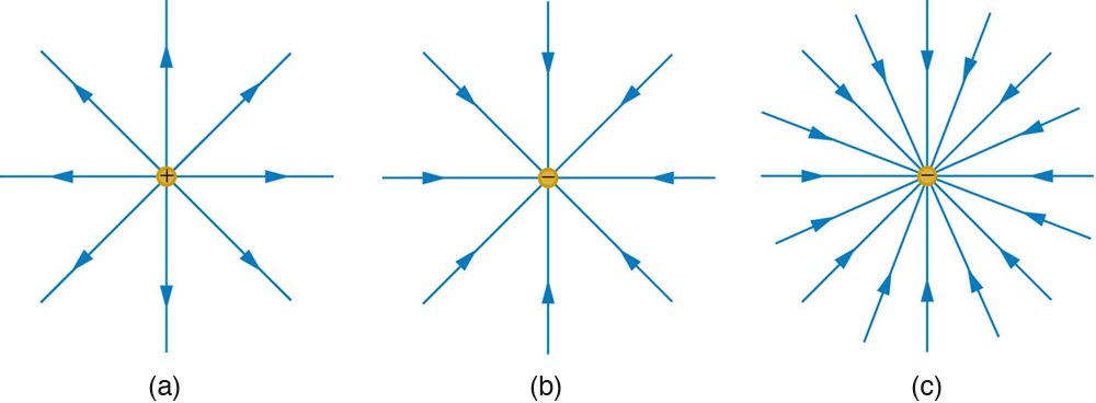
Note that the electric field is defined for a positive test charge , so that the field lines point away from a positive charge and toward a negative charge. (See Figure 18.23.) The electric field strength is exactly proportional to the number of field lines per unit area, since the magnitude of the electric field for a point charge is and area is proportional to . This pictorial representation, in which field lines represent the direction and their closeness (that is, their areal density or the number of lines crossing a unit area) represents strength, is used for all fields: electrostatic, gravitational, magnetic, and others.
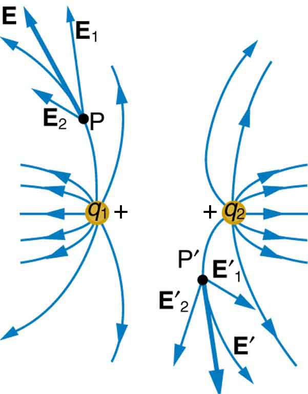
In many situations, there are multiple charges. The total electric field created by multiple charges is the vector sum of the individual fields created by each charge. The following example shows how to add electric field vectors.
Figure 18.25 shows how the electric field from two point charges can be drawn by finding the total field at representative points and drawing electric field lines consistent with those points. While the electric fields from multiple charges are more complex than those of single charges, some simple features are easily noticed.
For example, the field is weaker between like charges, as shown by the lines being farther apart in that region. (This is because the fields from each charge exert opposing forces on any charge placed between them.) (See Figure 18.25 and Figure 18.26(a).) Furthermore, at a great distance from two like charges, the field becomes identical to the field from a single, larger charge.
Figure 18.26(b) shows the electric field of two unlike charges. The field is stronger between the charges. In that region, the fields from each charge are in the same direction, and so their strengths add. The field of two unlike charges is weak at large distances, because the fields of the individual charges are in opposite directions and so their strengths subtract. At very large distances, the field of two unlike charges looks like that of a smaller single charge.
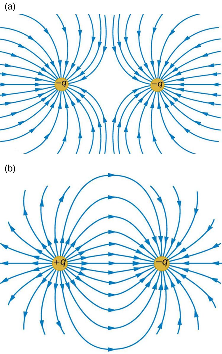
We use electric field lines to visualize and analyze electric fields (the lines are a pictorial tool, not a physical entity in themselves). The properties of electric field lines for any charge distribution can be summarized as follows:
- Field lines must begin on positive charges and terminate on negative charges, or at infinity in the hypothetical case of isolated charges.
- The number of field lines leaving a positive charge or entering a negative charge is proportional to the magnitude of the charge.
- The strength of the field is proportional to the closeness of the field lines—more precisely, it is proportional to the number of lines per unit area perpendicular to the lines.
- The direction of the electric field is tangent to the field line at any point in space.
- Field lines can never cross.
The last property means that the field is unique at any point. The field line represents the direction of the field; so if they crossed, the field would have two directions at that location (an impossibility if the field is unique).
Test Prep for AP Courses
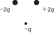
An electric dipole (with +2q and –2q as the two charges) is shown in the figure above. A third charge, −q is placed equidistant from the dipole charges. What will be the direction of the net force on the third charge?
- →
- ←
- ↓
- ↑
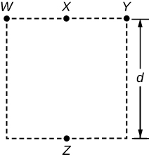
Four objects, each with charge +q, are held fixed on a square with sides of length d, as shown in the figure. Objects X and Z are at the midpoints of the sides of the square. The electrostatic force exerted by object W on object X is F. Use this information to answer questions 39–40.
What is the magnitude of force exerted by object W on Z?
- F/7
- F/5
- F/3
- F/2
(b)
What is the magnitude of the net force exerted on object X by objects W, Y, and Z?
- F/4
- F/2
- 9F/4
- 3F
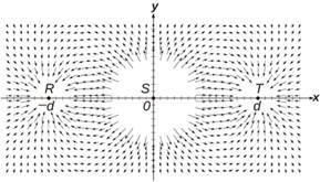
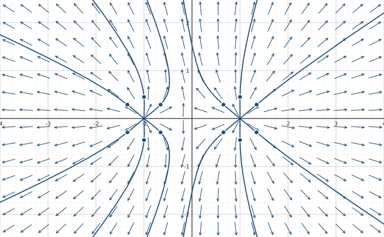
The figure above represents the electric field in the vicinity of three small charged objects, R, S, and T. The objects have charges −q, +2q, and −q, respectively, and are located on the x-axis at −d, 0, and d. Field vectors of very large magnitude are omitted for clarity.
(a) i) Briefly describe the characteristics of the field diagram that indicate that the sign of the charges of objects R and T is negative and that the sign of the charge of object S is positive.
ii) Briefly describe the characteristics of the field diagram that indicate that the magnitudes of the charges of objects R and T are equal and that the magnitude of the charge of object S is about twice that of objects R and T.
For the following parts, an electric field directed to the right is defined to be positive.
(b) On the axes below, sketch a graph of the electric field E along the x-axis as a function of position x.
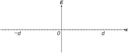
(c) Write an expression for the electric field E along the x-axis as a function of position x in the region between objects S and T in terms of q, d, and fundamental constants, as appropriate.
(d) Your classmate tells you there is a point between S and T where the electric field is zero. Determine whether this statement is true, and explain your reasoning using two of the representations from parts (a), (b), or (c).
(a) i) Field vectors near objects point toward negatively charged objects and away from positively charged objects.
(a) ii) The vectors closest to R and T are about the same length and start at about the same distance. We have that , so the charge on R is about the same as the charge on T. The closest vectors around S are about the same length as those around R and T. The vectors near S start at about 6 units away, while vectors near R and T start at about 4 units. We have that , so , and so the charge on S is about twice that on R and T.
(b)
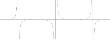
(c)
(d) The statement is not true. The vector diagram shows field vectors in this region with nonzero length, and the vectors not shown have even greater lengths. The equation in part (c) shows that, when , the denominator of the negative term is always greater than the denominator of the third term, but the numerator is the same. So the negative term always has a smaller magnitude than the third term and since the second term is positive the sum of the terms is always positive.
Section Summary
- Drawings of electric field lines are useful visual tools. The properties of electric field lines for any charge distribution are that:
- Field lines must begin on positive charges and terminate on negative charges, or at infinity in the hypothetical case of isolated charges.
- The number of field lines leaving a positive charge or entering a negative charge is proportional to the magnitude of the charge.
- The strength of the field is proportional to the closeness of the field lines—more precisely, it is proportional to the number of lines per unit area perpendicular to the lines.
- The direction of the electric field is tangent to the field line at any point in space.
- Field lines can never cross.
Conceptual Questions
Compare and contrast the Coulomb force field and the electric field. To do this, make a list of five properties for the Coulomb force field analogous to the five properties listed for electric field lines. Compare each item in your list of Coulomb force field properties with those of the electric field—are they the same or different? (For example, electric field lines cannot cross. Is the same true for Coulomb field lines?)
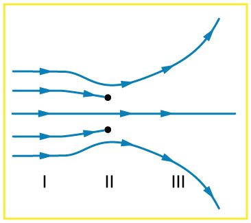
Figure 18.32 shows an electric field extending over three regions, labeled I, II, and III. Answer the following questions. (a) Are there any isolated charges? If so, in what region and what are their signs? (b) Where is the field strongest? (c) Where is it weakest? (d) Where is the field the most uniform?
Problem Exercises
(a) Sketch the electric field lines near a point charge . (b) Do the same for a point charge .
Sketch the electric field lines a long distance from the charge distributions shown in Figure 18.26 (a) and (b)
Figure 18.33 shows the electric field lines near two charges and . What is the ratio of their magnitudes? (b) Sketch the electric field lines a long distance from the charges shown in the figure.
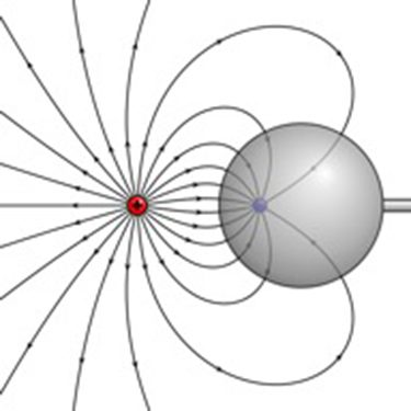
Sketch the electric field lines in the vicinity of two opposite charges, where the negative charge is three times greater in magnitude than the positive. (See Figure 18.33 for a similar situation).
Adapted from College Physics 2e by OpenStax (openstax.org), licensed under CC BY-NC-SA 4.0. Changes were made. License: CC-BY-NC-SA-4.0.